4.1 Uncertainty guided sampling

A sensible approach to improving quality of predictions is to: (a) estimate initial ML models, (b) produce a realistic estimate of prediction errors, and (c) revisit area and collect 2nd round samples that help at smallest possible costs significantly improve predictions. Logical focus of the 2nd round sampling could be thus on minimizing the overall prediction errors i.e. revising parts of the study area that shows the highest prediction errors / prediction problems (Fig. 2.7). This is exactly procedure that Stumpf et al. (2017) recommend in their paper and that they refer to as the “Uncertainty guided sampling”.

The 2nd round Uncertainty guided sampling can be implemented either by:

• Producing a strata based on the prediction error map (e.g. extrapolation areas / areas with highest uncertainty), then sampling only within that strata,
• Using the probability of exceeding threshold mapping accuracy to generate extra sampling points,

In both cases 2nd round points can be then added to the original training dataset and the model for the area can then be refitted (this procedure in data science is also referred to as “re-analysis”). Assuming that our initial model was unbiased, then even few tens of extra points could lead to significant reduction in RMSPE. In practice, we might have to also organize the 3rd round sampling until we finally reach some maximum possible accuracy (Hengl, Nussbaum, Wright, Heuvelink, & Gräler, 2018).

To generate 2nd round sampling for the Edgeroi dataset we can first estimate probability of prediction errors exceeding some threshold probability e.g. RMSE=0.2. We first load point data and prediction error map produced in the previous example using Ensemble Machine Learning:

data(edgeroi)
edgeroi.sp <- edgeroi$sites
coordinates(edgeroi.sp) <- ~ LONGDA94 + LATGDA94
proj4string(edgeroi.sp) <- CRS("+proj=longlat +ellps=GRS80 +towgs84=0,0,0,0,0,0,0 +no_defs")
edgeroi.sp <- spTransform(edgeroi.sp, CRS("+init=epsg:28355"))

The probability of exceeding some threshold, assuming normal distribution of prediction erros can be derived as:

t.RMSE = 0.2
edgeroi.error = readGDAL("./output/edgeroi_soc_rmspe.tif")
#> ./output/edgeroi_soc_rmspe.tif has GDAL driver GTiff 
#> and has 321 rows and 476 columns
edgeroi.error$inv.prob = 1/(1-2*(pnorm(edgeroi.error$band1/t.RMSE)-0.5)) 

next, we can generate a sampling plan using the spatstat package and the inverse probability of the pixels exceeding threshold uncertainty (f argument):

dens.var <- spatstat.geom::as.im(sp::as.image.SpatialGridDataFrame(edgeroi.error["inv.prob"]))
pnts.new <- spatstat.core::rpoint(50, f=dens.var)

So the new sampling plan, assuming adding only 50 new points would thus look like this:

plot(log1p(raster(edgeroi.error[c("inv.prob")])))
points(edgeroi.sp, pch="+", cex=.8, col="blue")
points(as(pnts.new, "SpatialPoints"), pch=19, cex=0.8, col="black")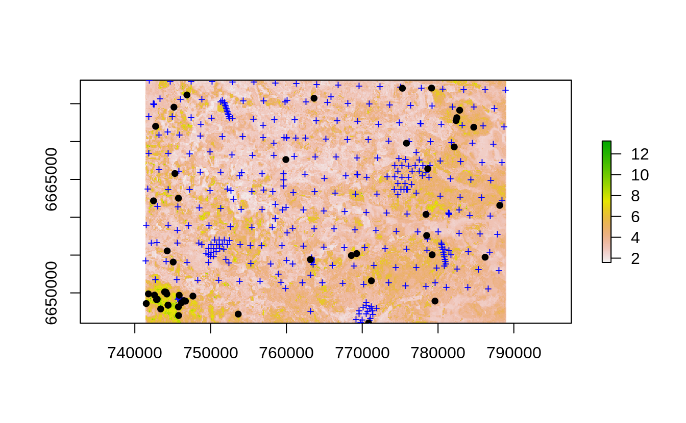

Figure 4.1: Uncertainty guided 2nd round sampling: locations of initial (+) and 2nd round points (dots).

This puts much higher weight at locations where the prediction errors are higher, however, technically speaking we finish still sampling points across the whole study area and, of course, including randomization.

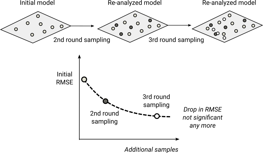
Figure 4.2: General scheme for re-sampling and re-analysis using uncertainty guided sampling principles.

By adding 2nd, 3rd round sampling we can imagine that the mapping accuracy / RMSE would gradually decrease following a decay function (e.g. RMSE = b0 * x ^ -b1) until some maximum possible accuracy is achieved. This way soil surveyor can optimize the predictions and reduce costs by minimizing number of additional samples i.e. it could be considered the shortest path to increasing the mapping accuracy without a need to start sampling from scratch.