5.1 Which sampling algorithm to choose?

In this tutorial we have demonstrated some main steps required to analyze existing sample designs (point patterns) and compare them with sampling algorithms such as the SRC, LHS and FSCS. Some general conclusions are:

• Understanding limitations of spatial samples used for ML is important. Diversity of tools now exist that allow for sampling diagnostics, especially to determine spatial clustering, potential extrapolation areas, to test Complete Spatial Randomness etc;
  
• Ensemble Machine Learning is at the order of magnitude more computational, but using combination of simple and complex base learners and spatial blocking seem to help produce models with less artifacts in extrapolation space and which report a more realistic mapping accuracy than if spatial clustering is ignored;
  
• The forestError package seems to provide a complete framework for uncertainty assessment and can be used to derive the prediction errors (RMSPE) per-pixel i.e. for each new prediction location; the average prediction error of the whole area is the mean prediction error that one can report to the users as the best unbiased estimate of the mean uncertainty;

Figure below shows differences between the above mentioned sampling algorithms in both geographical and feature spaces. In this case: actual sampling is significantly missing the whole cluster in feature space, while FSCS seems to show the highest spread in the feature space and by many authors is recognized as the most advantageous sampling design for predictive mapping (Ma, Brus, Zhu, Zhang, & Scholten, 2020). Such sampling diagnostics / comparisons geographical vs feature space help us detect any possible problems before we start running ML.

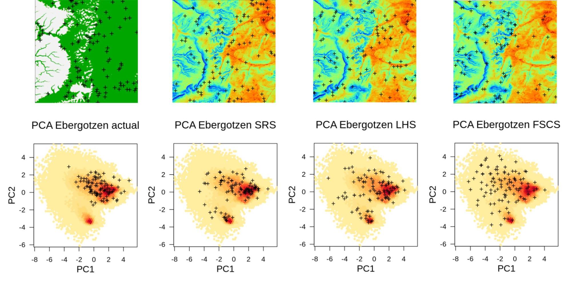
Figure 5.1: Summary comparison of sampling designs: convenience sampling (actual), Simple Random Sample (SRS), Latin Hypercube Sampling (LHS), and Feature Space Coverage Sampling (FSCS). Points shown in geographical (above) and feature space (below; with first 2 principal components as x, y coordinates).

5.2 Sampling in a new area

Recommended steps to prepare a sampling plan include:

1. Prepare all covariate layers (rasters) that you plan to use to fit predictive mapping models; import them to R;
2. Convert covariate layers to Principal Components using the landmap::spc function;
3. Cluster the feature space using the h2o.kmeans function; for smaller number of samples use number of clusters equal to number of sampling locations;
4. Generate a sampling design and export the points to GPX format so they can be imported to a hand-held GPS or similar. For fieldwork we recommend using the ViewRanger app which has useful functionality for field work including planning the optimal routes.

If you are collecting more than a few hundred points, then FSCS could become cumbersome and we hence recommend using LHS sampling. This sampling algorithm spreads points symmetrically in the feature space and ensures that the extrapolation (in feature space) is minimized.

5.3 ML on clustered point samples

Assuming that there is significant spatial and/or feature space clustering in training points, it appears that various blocking / Cross-Validation strategies, especially based on Ensemble ML help produce more balanced estimate of regression parameters and of the mapping accuracy. Incorporation of spatial proximity i.e.  autocorrelation has roots in the Generalized Least Squares methods (Venables & Ripley, 2002) and in the classical data science papers e.g. by Roberts et al. (2017). Ensemble ML with spatial blocking comes, however, at the costs of the order of magnitude higher computing costs.

In theory, even the most clustered point datasets can be used to fit predictive mapping models, however, it is then important to use modeling methods that account for clustering and prevent doing over-fitting and/or producing not realistic measures of mapping accuracy. Eventually, very biased point samples totally missing ≫50% of the feature / geographical space would be of limited use for producing predictions, but could still be used to get some initial estimates.

Wadoux, Heuvelink, de Bruin, & Brus (2021) shows that, assuming that training points are based on the probability sampling i.e. SRS, there is no need for spatial blocking i.e. regardless of the spatial dependence structure in the target variable, any subset of SRS would give an unbiased estimator of the mean population parameters. Many spatial statisticians hence argue that mapping accuracy can be determined only by collecting data using probability sampling (D. J. Brus, Kempen, & Heuvelink, 2011). Indeed, we also recommend to users of these tutorials to try your best to generate sampling designs using LHS, FSCS or at least SRS, as this ensures unbiased derivation of population parameters. Here the book by D. J. Brus (2021) seems to be a valuable resource as it also provides practical instructions for a diversity of data types.

If you have a dataset that you have used to test sampling and resampling, please share your experiences by posting an issue and/or providing a screenshot of your results.