1.1 Spatial sampling algorithms of interest

This chapter reviews some common approaches for preparing point samples for a study area that you are visiting for the first time and/or no previous samples or models are available. We focus on the following spatial sampling methods:

• Subjective or convenience sampling,
• Simple Random Sampling (SRS) (Bivand, Pebesma, & Rubio, 2013; Brus, 2021),
• Latin Hypercube Sampling (LHS) and its variants e.g. Conditioned LHS (Malone, Minansy, & Brungard, 2019; Minasny & McBratney, 2006),
• Feature Space Coverage Sampling (FSCS) (Goerg, 2013) and fuzzy k-means clustering (Hastie, Tibshirani, & Friedman, 2009),
• 2nd round sampling (Stumpf et al., 2017),

Our interest in this tutorials is in producing predictions (maps) of the target variable by employing regression / correlation between the target variable and multitude of features (raster layers), and where various Machine Learning techniques are used for training and prediction.

Once we collect enough training points in an area we can overlay points and GIS layers to produce a regression matrix or classification matrix, and which can then be used to generate spatial predictions i.e. produce maps. As a state-of-the-art we use the mlr framework for Ensemble Machine Learning as the key Machine Learning framework for predictive mapping. For an introduction to Ensemble Machine Learning for Predictive Mapping please refer to this tutorial.

1.2 Ebergotzen dataset

To test various sampling and mapping algorithms, we can use the Ebergotzen dataset available also via the plotKML package (Hengl, Roudier, Beaudette, & Pebesma, 2015):

set.seed(100)
library(plotKML)
library(sp)
library(viridis)
#> Loading required package: viridisLite
library(raster)
library(ggplot2)
data("eberg_grid25")
gridded(eberg_grid25) <- ~x+y
proj4string(eberg_grid25) <- CRS("+init=epsg:31467")

This dataset is described in detail in Böhner, Blaschke, & Montanarella (2008). It is a soil survey dataset with ground observations and measurements of soil properties including soil types. The study area is a perfect square 10×10 km in size.

We have previously derived number of additional DEM parameters directly using SAGA GIS (Conrad et al., 2015) and which we can add to the list of covariates:

eberg_grid25 = cbind(eberg_grid25, readRDS("./extdata/eberg_dtm_25m.rds"))
names(eberg_grid25)
#>  [1] "DEMTOPx"        "HBTSOLx"        "TWITOPx"        "NVILANx"       
#>  [5] "eberg_dscurv"   "eberg_hshade"   "eberg_lsfactor" "eberg_pcurv"   
#>  [9] "eberg_slope"    "eberg_stwi"     "eberg_twi"      "eberg_vdepth"  
#> [13] "PMTZONES"

so a total of 11 layers at 25-m spatial resolution, from which two layers (HBTSOLx and PMTZONES) are factors representing soil units and parent material units. Next, for further analysis, and to reduce data overlap, we can convert all primary variables to (numeric) principal components using:

eberg_spc = landmap::spc(eberg_grid25[-c(2,3)])
#> Converting PMTZONES to indicators...
#> Converting covariates to principal components...

which gives the a total of 14 PCs. The patterns in the PC components reflect a complex combination of terrain variables, lithological discontinuities (PMTZONES) and surface vegetation (NVILANx):

spplot(eberg_spc@predicted[1:3], col.regions=SAGA_pal[[1]])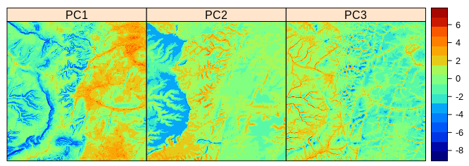

Figure 1.1: Principal Components derived using Ebergotzen dataset.

1.3 Simple Random Sampling

To generate a SRS with e.g. 100 points we can use the sp package spsample method:

rnd <- spsample(eberg_grid25[1], type="random", n=100)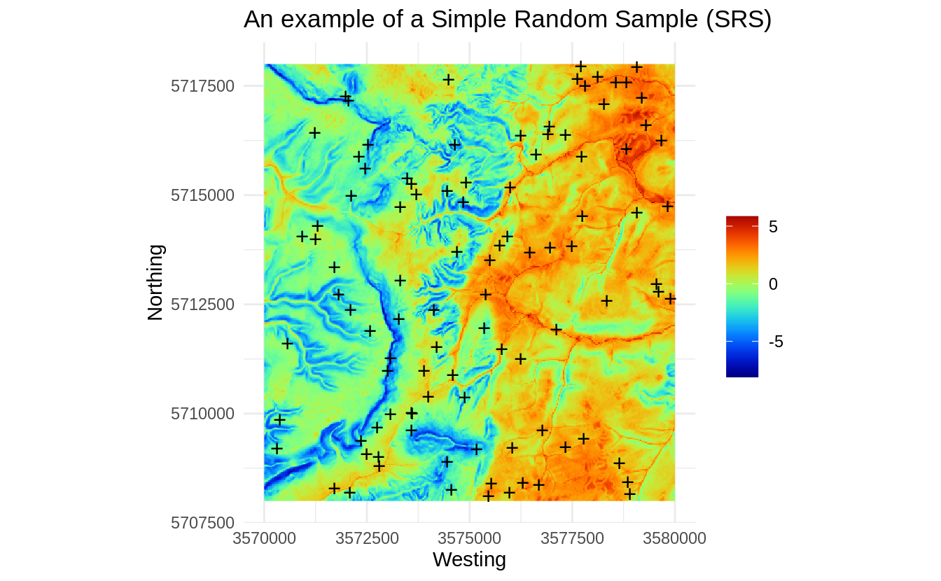

plot(raster(eberg_spc@predicted[1]), col=SAGA_pal[[1]])
points(rnd, pch="+")

Figure 1.2: An example of a Simple Random Sample (SRS).

This sample is generated purely based on the spatial domain, the feature space is completely ignored / not taken into account, hence we can check how well do these points represent the feature space using a density plot:

ov.rnd = sp::over(rnd, eberg_spc@predicted[,1:2])
library(hexbin)
library(grid)
reds = colorRampPalette(RColorBrewer::brewer.pal(9, "YlOrRd")[-1])
hb <- hexbin(eberg_spc@predicted@data[,1:2], xbins=60)
p <- plot(hb, colramp = reds, main='PCA Ebergotzen SRS')
pushHexport(p$plot.vp)
grid.points(ov.rnd[,1], ov.rnd[,2], pch="+")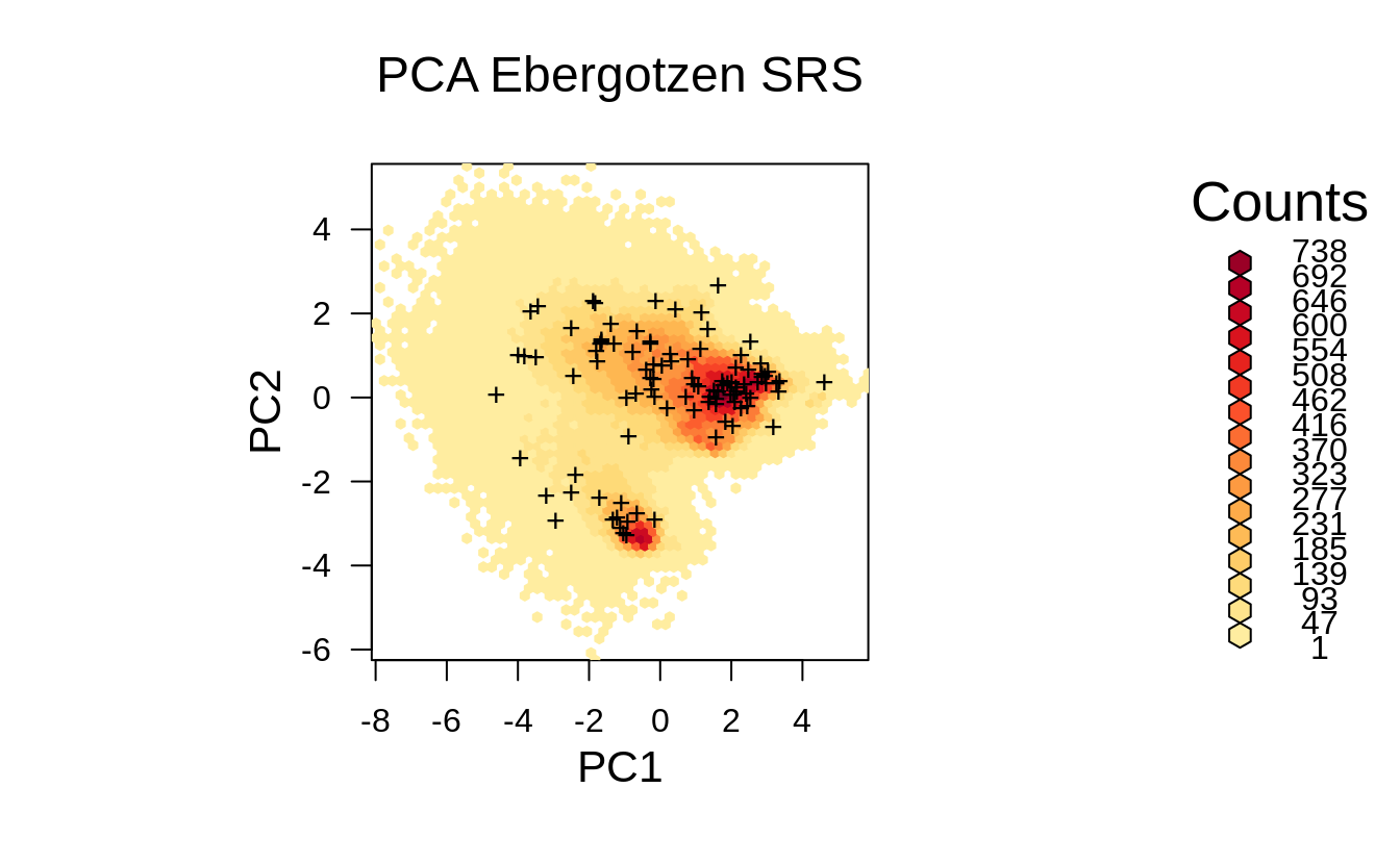

Figure 1.3: Distribution of the SRS points from the previous example in the feature space.

Visually, we do not directly see from Fig. 1.3 that the generated SRS maybe misses some important feature space, however if we zoom in, then we can notice that some parts of feature space (in this specific randomization) with high density are somewhat under-represented. Imagine if we reduce number of sampling points then we run even higher risk of missing some areas in the feature space by using SRS.

Next, we are interested in evaluating the occurrence probability of the SRS points based on the PCA components. To derive the occurrence probability we can use the maxlike package method (Royle, Chandler, Yackulic, & Nichols, 2012):

fm.cov <- stats::as.formula(paste("~", paste(names(eberg_spc@predicted[1:4]), collapse="+")))
ml <- maxlike::maxlike(formula=fm.cov, rasters=raster::stack(eberg_spc@predicted[1:4]), 
                       points=rnd@coords, method="BFGS", removeDuplicates=TRUE, savedata=TRUE)
ml.prob <- predict(ml)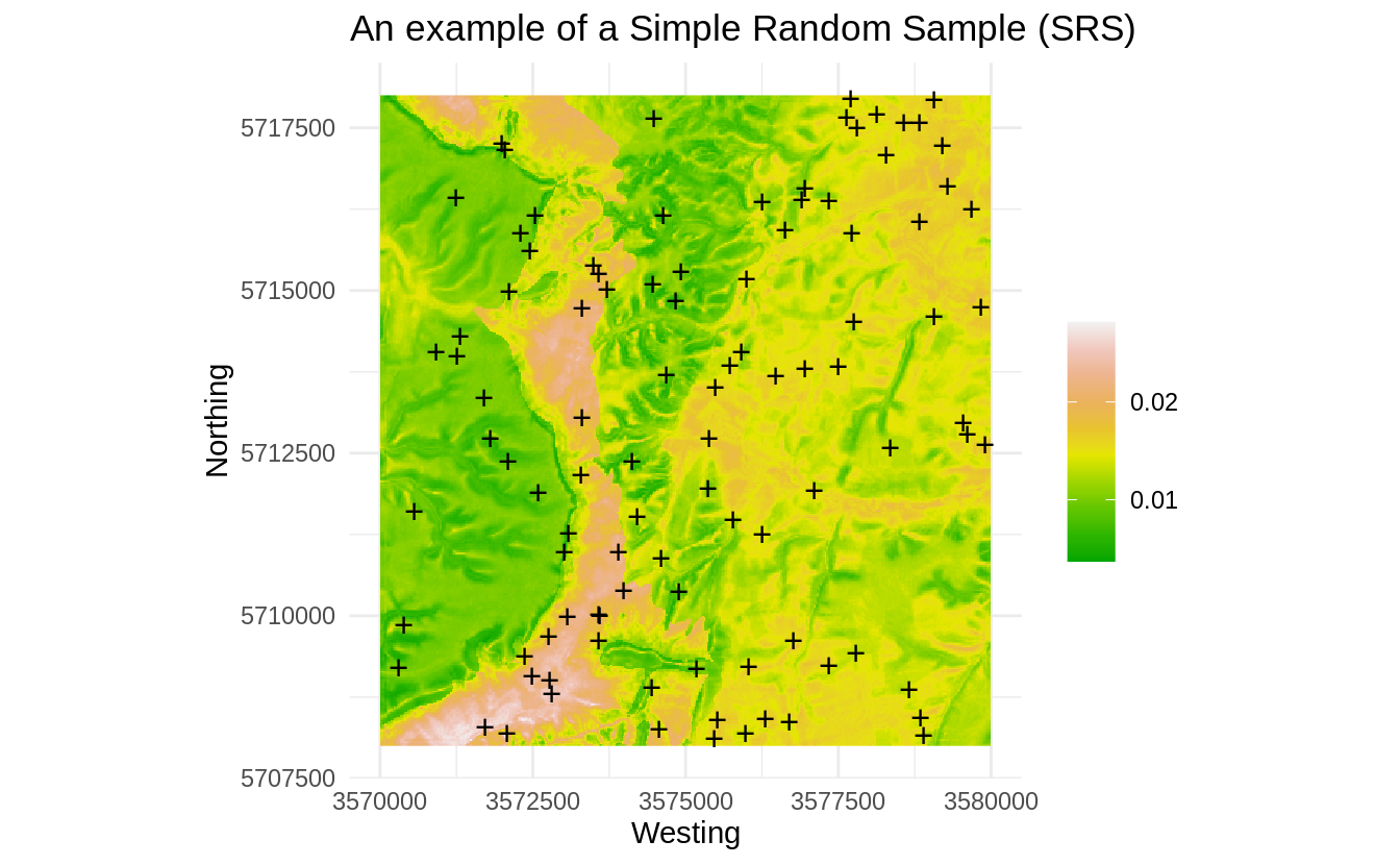

plot(ml.prob)
points(rnd@coords, pch="+")

Figure 1.4: Occurrence probability for SRS derived using the maxlike package.

Note: for the sake of reducing the computing intensity we focus on the first four PCs. In practice, feature space analysis can be quite computational and we recommend using parallelized versions within an High Performance Computing environments to run such analysis.

Fig. 1.4 shows that, by accident, some parts of the feature space might be somewhat under-represented (areas with low probability of occurrence on the map). Note however that occurrence probability for this dataset is overall very low (<0.05), indicating that distribution of points is not much correlated with the features. This specific SRS is thus probably satisfactory also for feature space analysis: the SRS points do not seem to group (which would in this case be by accident) and hence maxlike gives very low probability of occurrence.

We can repeat SRS many times and then see if the clustering of points gets more problematic, but as you can image, in practice for large number of samples it is a good chance that all features would get well represented also in the feature space even though we did not include feature space variables in the production of the sampling plan.

We can now also load the actual points collected for the Ebergotzen case study:

data(eberg)
eberg.xy <- eberg[,c("X","Y")]
coordinates(eberg.xy) <- ~X+Y
proj4string(eberg.xy) <- CRS("+init=epsg:31467")
ov.xy = sp::over(eberg.xy, eberg_grid25[1])
eberg.xy = eberg.xy[!is.na(ov.xy$DEMTOPx),]
sel <- sample.int(length(eberg.xy), 100)
eberg.smp = eberg.xy[sel,]

To quickly estimate spread of points in geographical and feature spaces, we can also use the function spsample.prob that calls both the kernel density function from the spatstat package, and derives the probability of occurrence using the maxlike package:

iprob <- landmap::spsample.prob(eberg.smp, eberg_spc@predicted[1:4])
#> Deriving kernel density map using sigma 1010 ...
#> Deriving inclusion probabilities using MaxLike analysis...

In this specific case, the actual sampling points are much more clustered, so if we plot the two occurrence probability maps derived using maxlike next to each other we get:

op <- par(mfrow=c(1,2))
plot(raster(iprob$maxlike), zlim=c(0,1))
points(eberg.smp@coords, pch="+")
plot(ml.prob, zlim=c(0,1))
points(rnd@coords, pch="+")
par(op)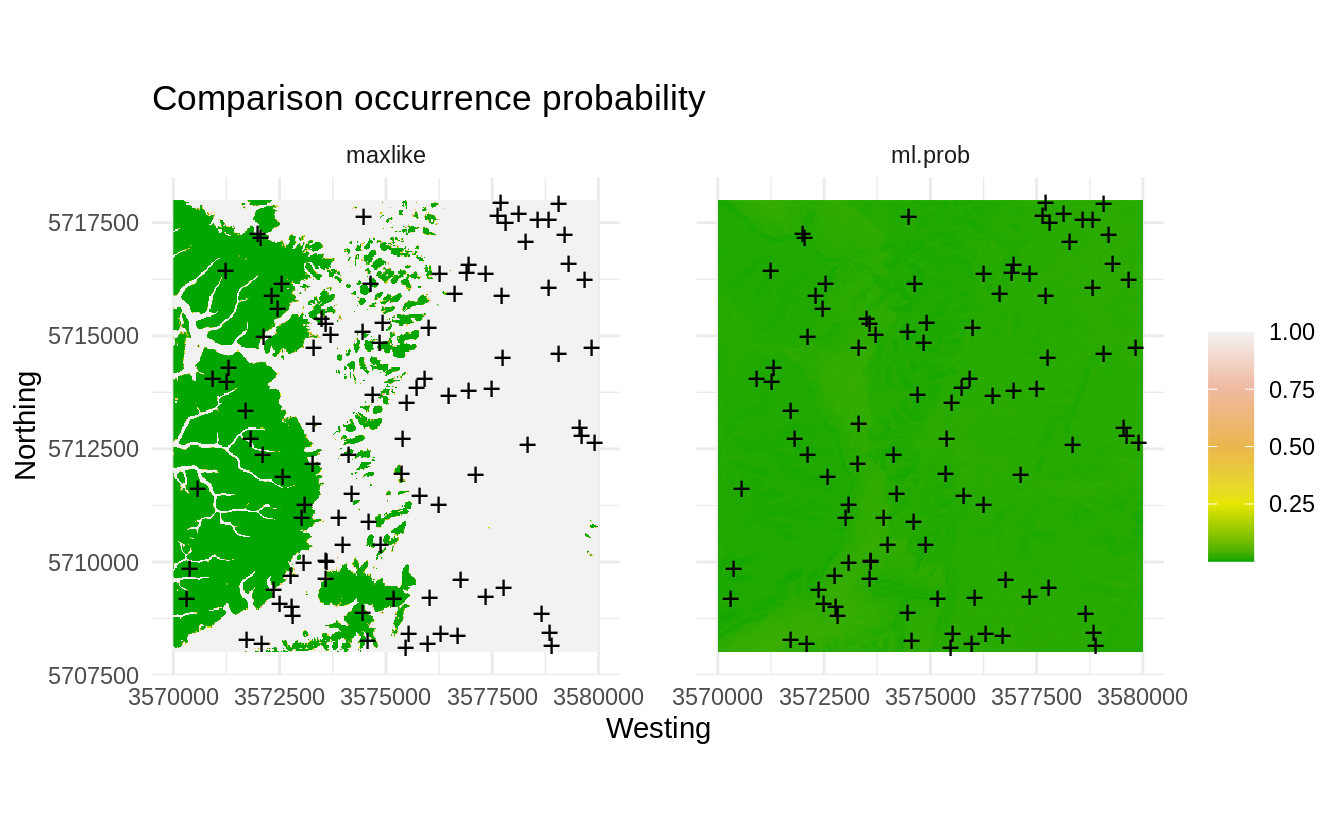

Figure 1.5: Comparison occurrence probability for actual and SRS samples derived using the maxlike package.

The map on the left clearly indicates that most of the sampling points are basically preferentially located in the plain area, while the hillands are systematically under-sampled. This we can also cross-check by reading the description of the dataset in Böhner, Blaschke, & Montanarella (2008):

• the Ebergotzen soil survey points focus on agricultural land only,
  
• no objective sampling design has been used, hence some points are clustered,

This is also clearly visible from the feature map plot where one part of the feature space seem to be completely omitted from sampling:

ov2.rnd = sp::over(eberg.smp, eberg_spc@predicted[,1:2])
p <- plot(hb, colramp = reds, main='PCA Ebergotzen actual')
pushHexport(p$plot.vp)
grid.points(ov2.rnd[,1], ov2.rnd[,2], pch="+")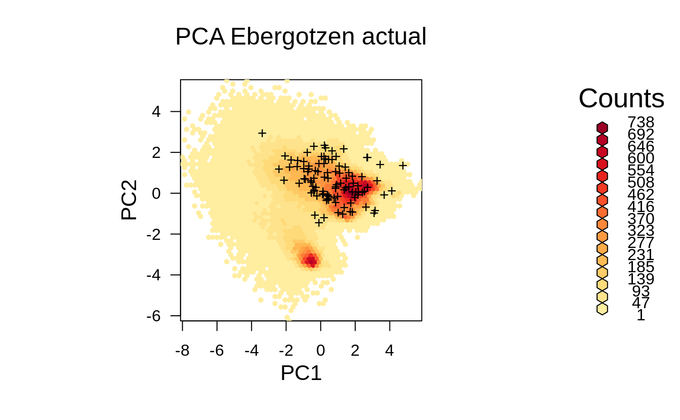

Figure 1.6: Distribution of the actual survey points from the previous example displayed in the feature space.

1.4 Latin Hypercube Sampling

In the previous example we have shown how to implement SRS and then also evaluate it against feature layers. Often SRS represent very well feature space so it can be directly used for Machine Learning and with a guarantee of not making too much bias
in predictions. To avoid, however, risk of missing out some parts of the feature space, and also to try to optimize allocation of points, we can generate a sample using the Latin Hypercube Sampling (LHS) method. In a nutshell, LHS methods are based on dividing the Cumulative Density Function (CDF) into n equal partitions, and then choosing a random data point in each partition, consequently:

• CDF of LHS samples matches the CDF of population (hence unbiased representation),
  
• Extrapolation in the feature space should be minimized,

Latin Hypercube and sampling optimization using LHS is explained in detail in Minasny & McBratney (2006) and Shields & Zhang (2016). The lhs package also contains numerous examples of how to implement for (non-spatial) data.

Here we use an implementation of the LHS available in the clhs package (P. Roudier, 2021):

library(clhs)
rnd.lhs = clhs::clhs(eberg_spc@predicted[1:4], size=100, iter=100, progress=FALSE)

This actually implements the so-called “Conditional LHS” (Minasny & McBratney, 2006), and can get quite computational for large stack of rasters, hence we manually limit the number of iterations to 100.

We can plot the LHS sampling plan:

plot(raster(eberg_spc@predicted[1]), col=SAGA_pal[[1]])
points(rnd.lhs@coords, pch="+")

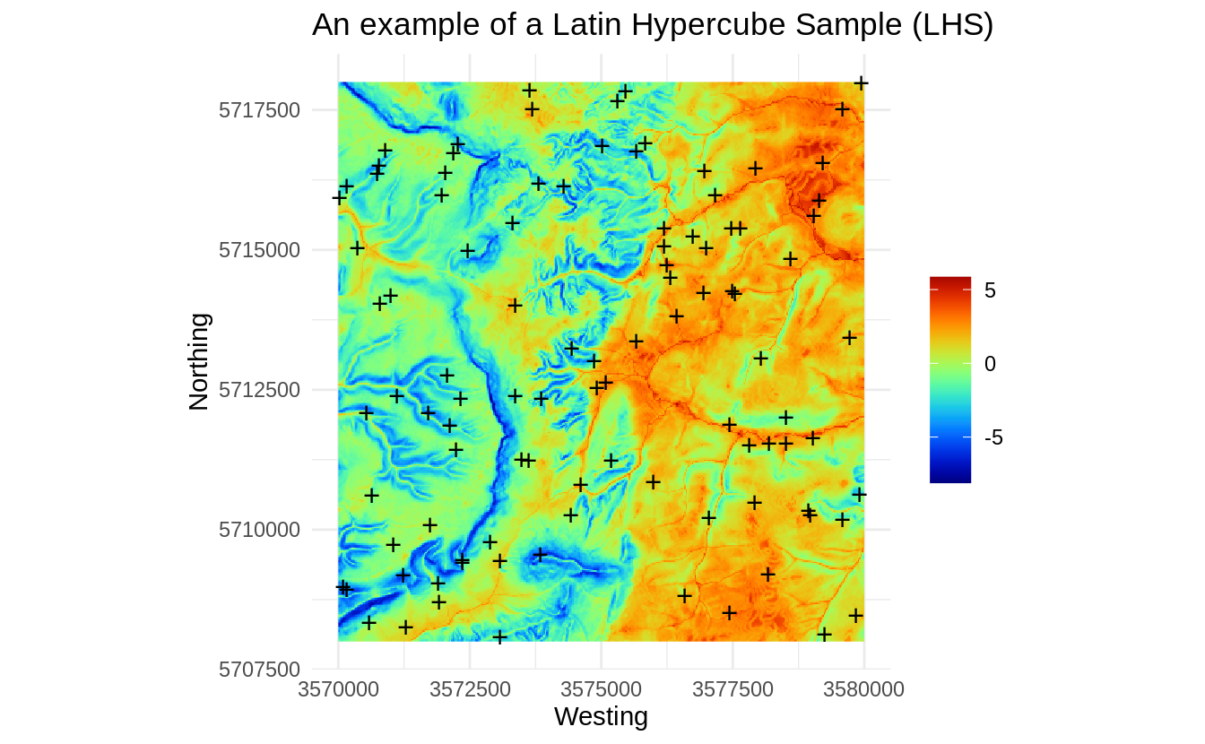
Figure 1.7: An example of a Latin Hypercube Sample (LHS).

p <- plot(hb, colramp = reds, main='PCA Ebergotzen LHS')
pushHexport(p$plot.vp)
grid.points(rnd.lhs$PC1, rnd.lhs$PC2, pch="+")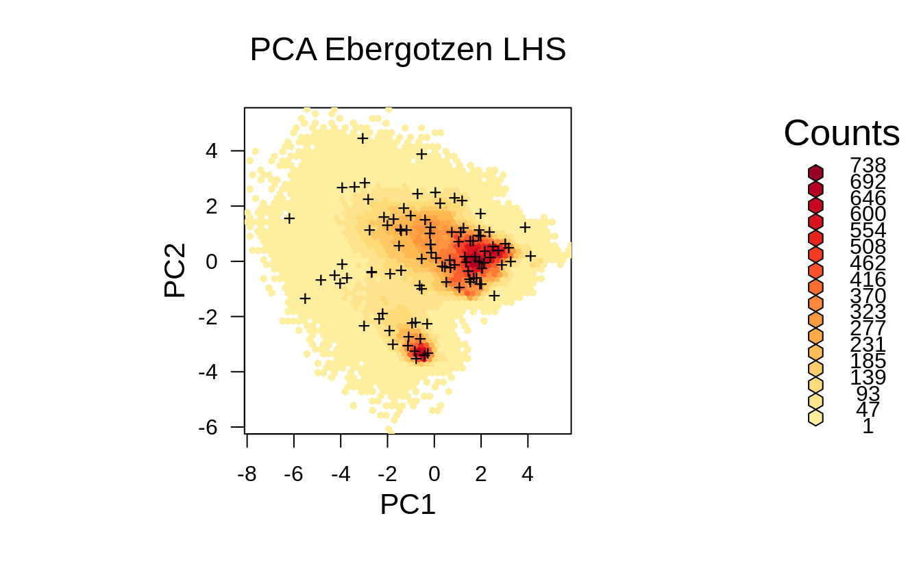

Figure 1.8: Distribution of the LHS points from the previous example displayed in the feature space.

Although in principle we might not see any difference in the point pattern between SRS and LHS, the feature space plot clearly shows that LHS covers systematically feature space map, i.e. we would have a relatively low risk of missing out some important features as compared to Fig. 1.6.

Thus the main advantages of the LHS are:

• it ensures that feature space is represented systematically i.e. it is optimized for Machine Learning using the specific feature layers;
  
• it is an Independent Identically Distributed (IID) sampling design;
  
• thanks to the clhs package, also the survey costs raster layer can be integrated to still keep systematic spread, but reduce survey costs as much as possible (Pierre Roudier, Beaudette, & Hewitt, 2012);

1.5 Feature Space Coverage Sampling

The Feature Space Coverage Sampling (FSCS) is described in detail in Brus (2019). In a nutshell, FSCS aims at optimal coverage of the feature space which is achieved by minimizing the average distance of the population units (raster cells) to the nearest sampling units in the feature space represented by the raster layers (Ma, Brus, Zhu, Zhang, & Scholten, 2020).

To produce FSCS point sample we can use function kmeanspp of package LICORS (Goerg, 2013). First we partition the feature space cube to e.g. 100 clusters. We then select raster cells with the shortest scaled Euclidean distance in covariate-space to the centres of the clusters as the sampling units:

library(LICORS)
library(fields)
fscs.clust <- kmeanspp(eberg_spc@predicted@data[,1:4], k=100, iter.max=100)
D <- fields::rdist(x1 = fscs.clust$centers, x2 = eberg_spc@predicted@data[,1:4])
units <- apply(D, MARGIN = 1, FUN = which.min)
rnd.fscs <- eberg_spc@predicted@coords[units,]

Note: the k-means++ algorithm is of most interest for small sample sizes: “for large sample sizes the extra time needed for computing the initial centres can become substantial and may not outweigh the larger number of starts that can be afforded with the usual k-means algorithm for the same computing time” (Brus, 2021). The kmeanspp algorithm from the LICORS package is unfortunately quite computational and is in principle not recommended for large grids / to generate large number of samples. Instead, we recommend clustering feature space using the h2o.kmeans function from the h2o package, which is also suitable for larger datasets with computing running in parallel:

library(h2o)
h2o.init(nthreads = -1)
#> 
#> H2O is not running yet, starting it now...
#> 
#> Note:  In case of errors look at the following log files:
#>     /tmp/Rtmpoy1T4t/file136956636dd7/h2o_tomislav_started_from_r.out
#>     /tmp/Rtmpoy1T4t/file136935079fd2/h2o_tomislav_started_from_r.err
#> 
#> 
#> Starting H2O JVM and connecting: .. Connection successful!
#> 
#> R is connected to the H2O cluster: 
#>     H2O cluster uptime:         2 seconds 226 milliseconds 
#>     H2O cluster timezone:       Europe/Amsterdam 
#>     H2O data parsing timezone:  UTC 
#>     H2O cluster version:        3.30.0.1 
#>     H2O cluster version age:    1 year, 9 months and 13 days !!! 
#>     H2O cluster name:           H2O_started_from_R_tomislav_vru837 
#>     H2O cluster total nodes:    1 
#>     H2O cluster total memory:   15.71 GB 
#>     H2O cluster total cores:    32 
#>     H2O cluster allowed cores:  32 
#>     H2O cluster healthy:        TRUE 
#>     H2O Connection ip:          localhost 
#>     H2O Connection port:        54321 
#>     H2O Connection proxy:       NA 
#>     H2O Internal Security:      FALSE 
#>     H2O API Extensions:         Amazon S3, XGBoost, Algos, AutoML, Core V3, TargetEncoder, Core V4 
#>     R Version:                  R version 4.0.2 (2020-06-22)
#> Warning in h2o.clusterInfo(): 
#> Your H2O cluster version is too old (1 year, 9 months and 13 days)!
#> Please download and install the latest version from http://h2o.ai/download/
df.hex <- as.h2o(eberg_spc@predicted@data[,1:4], destination_frame = "df")
#> 
  |                                                                            
  |                                                                      |   0%
  |                                                                            
  |======================================================================| 100%
km.nut <- h2o.kmeans(training_frame=df.hex, k=100, keep_cross_validation_predictions = TRUE)
#> 
  |                                                                            
  |                                                                      |   0%
  |                                                                            
  |=======                                                               |  10%
  |                                                                            
  |======================================================================| 100%
#km.nut

Note: in the example above, we have manually set the number of clusters to 100, but the number of clusters could be also derived using some optimization procedure. Next, we predict the clusters and plot the output:

m.km <- as.data.frame(h2o.predict(km.nut, df.hex, na.action=na.pass))
#> 
  |                                                                            
  |                                                                      |   0%
  |                                                                            
  |======================================================================| 100%

We can save the class centers (if needed for any further analysis):

class_df.c = as.data.frame(h2o.centers(km.nut))
names(class_df.c) = names(eberg_spc@predicted@data[,1:4])
str(class_df.c)
#> 'data.frame':    100 obs. of  4 variables:
#>  $ PC1: num  -0.508 -2.418 -5.305 1.329 -3.728 ...
#>  $ PC2: num  1.39 -4.52 1.42 2.03 1.85 ...
#>  $ PC3: num  0.0559 -3.3784 -1.7385 2.8903 3.3391 ...
#>  $ PC4: num  1.85 -2.72 -1.59 -2.26 3.85 ...
#write.csv(class_df.c, "NCluster_100_class_centers.csv")

To select sampling points we use the minimum distance to class centers (Brus, 2021):

D <- fields::rdist(x1 = class_df.c, x2 = eberg_spc@predicted@data[,1:4])
units <- apply(D, MARGIN = 1, FUN = which.min)
rnd.fscs <- eberg_spc@predicted@coords[units,]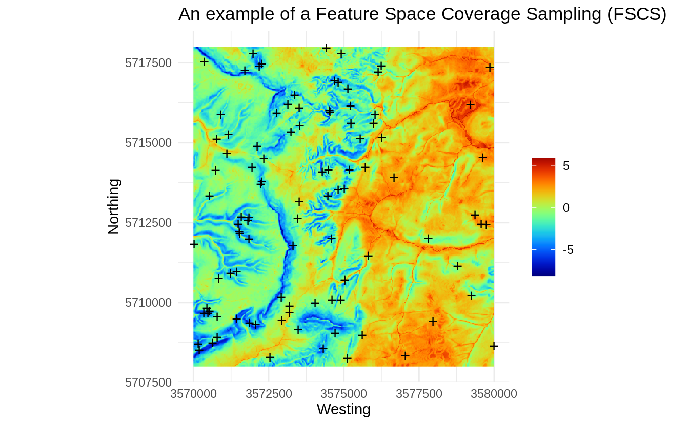

plot(raster(eberg_spc@predicted[1]), col=SAGA_pal[[1]])
points(rnd.fscs, pch="+")

Figure 1.9: An example of a Feature Space Coverage Sampling (FSCS).

Visually, FSCS seem to add higher spatial density of points in areas where there is higher complexity. The h2o.kmeans algorithm stratifies area into most possible homogeneous units (in the example above, large plains in the right part of the study area are relatively homogeneous, hence the sampling intensity in there areas drops significantly when visualized in the geographical space), and the points are then allocated per each strata.

p <- plot(hb, colramp = reds, main='PCA Ebergotzen FSCS')
pushHexport(p$plot.vp)
grid.points(eberg_spc@predicted@data[units,"PC1"], eberg_spc@predicted@data[units,"PC2"], pch="+")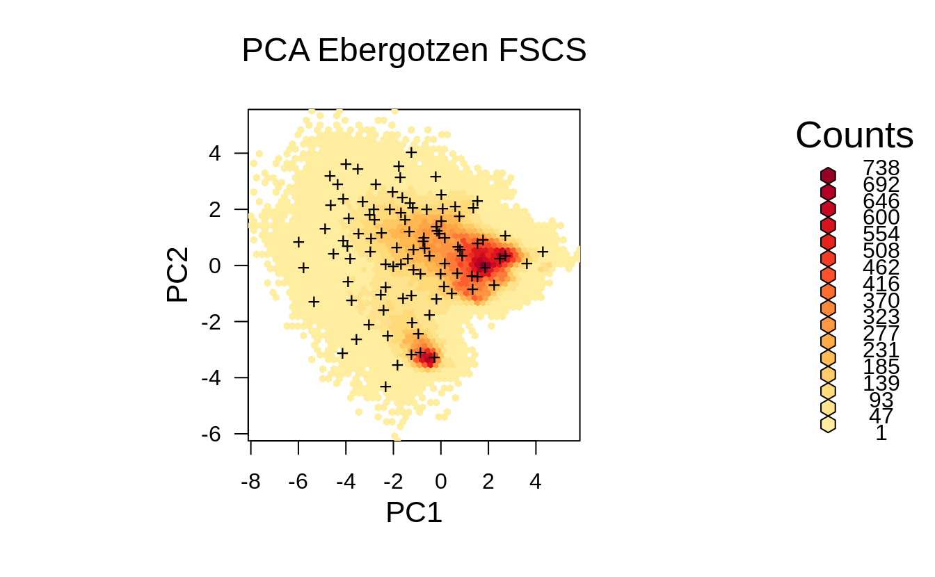

Figure 1.10: Distribution of the FSCS points from the previous example displayed in the feature space.

The FSCS sampling pattern in feature space looks almost as grid sampling in feature space. FSCS seems to put more effort on sampling at the edges on the feature space in comparison to LHS and SRS, and hence can be compared to classical response surface designs such as D-optimal designs (Hengl, Rossiter, & Stein, 2004).

h2o.shutdown(prompt = FALSE)

1.6 Summary points

In the previous examples we have shown differences between SRS, LHS and FSCS. SRS and LHS are IID sampling methods and as long as the number of samples is large and the study area is complex, it is often difficult to notice or quantify any under- or over-sampling. Depending on which variant of FSCS we implement, FSCS can result in higher spatial spreading especially if a study area consists of a combination of a relatively homogeneous and complex terrain units.

The Ebergotzen dataset (existing point samples) clearly shows that the “convenience surveys” can show significant clustering and under-representation of feature space (Fig. 1.6). Consequently, these sampling bias could lead to:

• Bias in estimating regression parameters i.e. overfitting;
  
• Extrapolation problems due to under-representation of feature space;
  
• Bias in estimating population parameters of the target variable;

The first step to deal with these problems is to detect them, second is to try to implement a strategy that prevents from model overfitting. Some possible approaches to deal with such problems are addressed in the second part of the tutorial.

LHS and FSCS are recommended sampling methods if the purpose of sampling is to build regression or classification models using multitude of (terrain, climate, land cover etc) covariate layers. Ma, Brus, Zhu, Zhang, & Scholten (2020) compared LHS to FSCS for mapping soil types and concluded that FSCS results in better mapping accuracy, most likely because FSCS spreads points better in feature space and hence in their case studies that seem to have helped with producing more accurate predictions. Yang et al. (2020) also report that LHS helps improve accuracy only for the large size of points.

The h2o.kmeans algorithm is suited for large datasets, but nevertheless to generate ≫100 clusters using large number of raster layers could become RAM consuming and is maybe not practical for operational sampling. An alternative would be to reduce number of clusters and select multiple points per cluster.

In the case of doubt which method to use LHS or FSCS, we recommend the following simple rules of thumb:

• If your dataset contains relatively smaller-size rasters and the targeted number of sampling points is relatively small (e.g. ≪1000), we recommend using the FSCS algorithm;
  
• If your project requires large number of sampling points (≫100), then you should probably consider using the LHS algorithm;

In general, as the number of sampling points starts growing, differences between SRS (no feature space) and LHS becomes minor, which can also be witnessed visually (basically it becomes difficult to tell the difference between the two). SRS could, however, by accident miss some important parts of the feature space, so in principle it is still important to use either LHS or FSCS algorithms to prepare sampling locations for ML where objective is to fit regression and/or classification models using ML algorithms.

To evaluate potential sampling clustering and pin-point under-represented areas one can run multiple diagnostics:

1. In geographical space:
   1. kernel density analysis using the spatstat package, then determine if some parts of the study area have systematically higher density;
      
   2. testing for Complete Spatial Randomness (Schabenberger & Gotway, 2005) using e.g. spatstat.core::mad.test and/or dbmss::Ktest;
      
2. In feature space:
   1. occurrence probability analysis using the maxlike package;
   2. unsupervised clustering of the feature space using e.g. h2o.kmeans, then determining if any of the clusters are significantly under-represented / under-sampled;
      
   3. estimating Area of Applicability based on similarities between training prediction and feature spaces (Meyer & Pebesma, 2021);

Plotting generated sampling points both on a map and feature space map helps detect possible extrapolation problems in a sampling design (Fig. 1.6). If you detect problems in feature space representation based on an existing point sampling set, you can try to reduce those problems by adding additional samples e.g. through covariate space infill sampling (Brus, 2021) or through 2nd round sampling and then re-analysis. These methods are discussed in further chapters.