2  Resampling methods for Machine Learning
You are reading the work-in-progress Spatial Sampling and Resampling for Machine Learning. This chapter is currently currently draft version, a peer-review publication is pending. You can find the polished first edition at https://opengeohub.github.io/spatial-sampling-ml/.
2.1 Resampling and Cross-Validation
In the previous examples we have demonstrated how to prepare sampling designs for your own study area assuming no other point data is available. We have also demonstrated how to run some sampling representation diagnostics to detect potential problems especially in the feature space. In the next sections we will focus on how to use different resampling methods i.e. cross-validation strategies (Roberts et al., 2017) to help reduce problems such as:
-
overfitting i.e. producing models that are biased and/or over-optimistic;
-
missing out covariates that are important but possibly shadowed by the covariates
over-selected due to overfitting;
-
producing poor extrapolation i.e. generating artifacts or blunders in predictions;
- over-/under-estimating mapping accuracy i.e. producing a biased estimate of model performance including;
Resamping methods are discussed in detail in Hastie, Tibshirani, & Friedman (2009), Kuhn & Johnson (2013) and Roberts et al. (2017), and is also commonly implemented in many statistical and machine learning packages such as the caret or mlr. Spatial resampling methods are discussed in detail in Lovelace, Nowosad, & Muenchow (2019).
For an introduction to Cross-Validation please refer to this tutorial and the “Data Analysis and Prediction Algorithms with R” chapters on cross validation. For an introduction to spatial Cross-Validation refer to the “Geocomputation with R” book.
It can be said that, in general, purpose of Machine Learning for predictive mapping is to try to produce Best Unbiased Predictions (BUPS) of the target variable and the associated uncertainty (e.g. prediction error). BUPS is commonly implemented through: (1) selecting the Best Unbiased Predictor (Venables & Ripley, 2002), (2) selecting the optimal subset of covariates and model parameters (usually by iterations), (3) applying predictions and providing an estimate of the prediction uncertainty i.e. estimate of the prediction errors / prediction intervals for a given probability distribution. In this tutorial the path to BUPS we use includes:
- Ensemble Machine Learning using stacking approach with 5-fold Cross-Validation with a meta-learner i.e. an independent model correlating competing base-learners with the target variable (Bischl et al., 2016; Polley & Van Der Laan, 2010),
- Estimating prediction errors using quantile regression Random Forest (Lu & Hardin, 2021),
The reasoning for using Ensemble ML for predictive mapping is explained in detail in this tutorial, and it’s advantages for minimizing extrapolation effects in this medium post.
2.2 Resampling training points using declustering
In the previous example we have shown that the actual soil survey points for Ebergotzen are somewhat spatially clustered, they under-sample forest areas / hillands. In statistical term these sampling points are geographically unbalanced i.e. non-IID. If we plot the original sampling points (N=2780) we see high spatial clustering of samples:
library(rgdal)
library(raster)
library(plotKML)
library(landmap)
library(mlr)
data("eberg_grid25")
gridded(eberg_grid25) <- ~x+y
proj4string(eberg_grid25) <- CRS("+init=epsg:31467")
eberg_grid25 = cbind(eberg_grid25, readRDS("./extdata/eberg_dtm_25m.rds"))
eberg_spc = landmap::spc(eberg_grid25[-c(2,3)])
#> Converting PMTZONES to indicators...
#> Converting covariates to principal components...
data(eberg)
eberg.xy <- eberg[,c("X","Y")]
coordinates(eberg.xy) <- ~X+Y
proj4string(eberg.xy) <- CRS("+init=epsg:31467")
ov.xy = sp::over(eberg.xy, eberg_grid25[1])
eberg.xy = eberg.xy[!is.na(ov.xy$DEMTOPx),]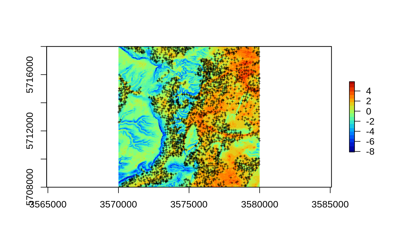
Figure 2.1: All sampling points available for Ebergotzen case study.
If we ignore that property of the data and directly fit a predictive model for e.g. top-soil clay content using e.g. random forest (Wright & Ziegler, 2017) we get:
library(ranger)
rm.eberg = cbind(eberg[!is.na(ov.xy$DEMTOPx),], sp::over(eberg.xy, eberg_spc@predicted))
cly.fm = as.formula(paste0("CLYMHT_A ~ ", paste0("PC", 1:13, collapse = "+")))
sel.cly = complete.cases(rm.eberg[,all.vars(cly.fm)])
rm.cly = rm.eberg[sel.cly,]
rf.cly = ranger::ranger(cly.fm, data=rm.cly)
rf.cly
#> Ranger result
#>
#> Call:
#>  ranger::ranger(cly.fm, data = rm.cly)
#>
#> Type:                             Regression
#> Number of trees:                  500
#> Sample size:                      2776
#> Number of independent variables:  13
#> Mtry:                             3
#> Target node size:                 5
#> Variable importance mode:         none
#> Splitrule:                        variance
#> OOB prediction error (MSE):       53.23538
#> R squared (OOB):                  0.6081801
This shows an RMSE of about 7.3% and an R-square of about 0.61. The problem of this accuracy measure is that with this Random Forest model we ignore spatial clustering of points, hence both the model and the accuracy metric could be over-optimistic (Meyer, Reudenbach, Hengl, Katurji, & Nauss, 2018; Roberts et al., 2017). Because we are typically interested in how does the model perform over the WHOLE area of interest, not only in comparison to out-of-bag points, to reduce overfitting or any bias in the BUPS we need to apply some adjustments.
Strategy #1 for producing more objective estimate of model parameters is to
resample sampling points by forcing as much as possible equal sampling intensity
(hence mimicking the SRS), then observe performance of the model accuracy.
We can implement such spatial resampling using the sample.grid function,
which basically resamples the existing point samples with an objective of producing
a sample more similar to SRS. This type of subsetting can be run M times and
then an ensemble model can be produced in which each individual model is based
on spatially balanced samples. These are not true SRS samples but we can refer
to them as the pseudo-SRS samples as they would probably pass all Spatial
Randomness tests.
In R we can implement spatial resampling using the following three steps. First, we generate e.g. 10 random subsets where the sampling intensity of points is relatively homogeneous:
eberg.sp = SpatialPointsDataFrame(eberg.xy, rm.eberg[c("ID","CLYMHT_A")])
sub.lst = lapply(1:10, function(i){landmap::sample.grid(eberg.sp, c(500, 500), n=2)})
This randomly subsets each 500-m block to max 2 points i.e. trims down the densely sampled points to produce a relatively balanced spatial sampling intensity. We can check that the training point sample looks more like a SRS or similar.
l1 <- list("sp.points", sub.lst[[1]]$subset, pch="+", col="black")
spplot(sub.lst[[1]]$grid, scales=list(draw=TRUE),
   col.regions="grey", sp.layout=list(l1), colorkey=FALSE)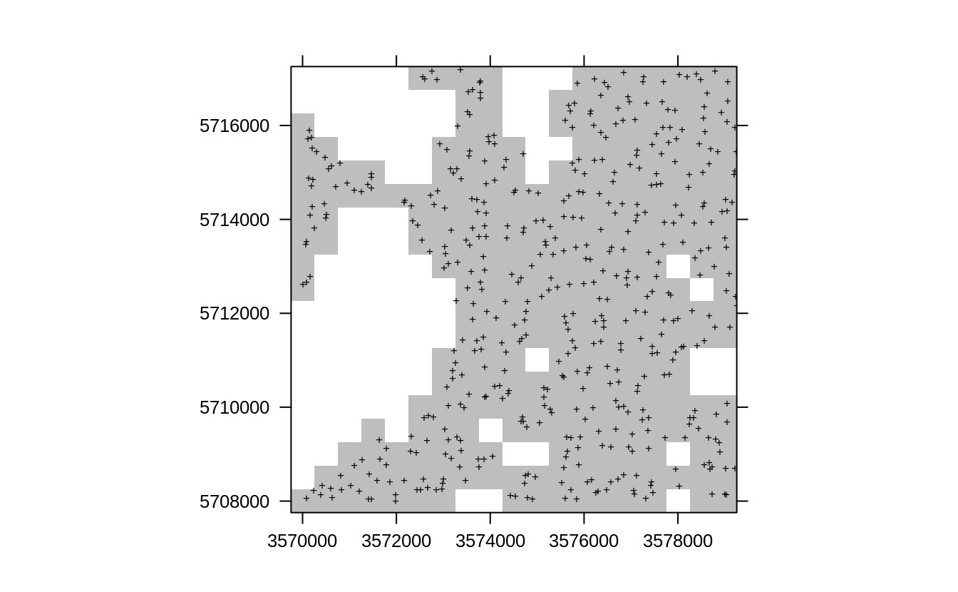
Figure 2.2: Resampling original points using sample.grid function, which produces a sample with similar properties such as SRS.
Second, we can fit a list of random forest models using 10 random draws mimicking some IID sampling:
rf.cly.lst = lapply(1:length(sub.lst), function(i){
        x <- rm.eberg[which(rm.eberg$ID %in% sub.lst[[i]]$subset$ID),];
        x <- x[complete.cases(x[,all.vars(cly.fm)]),];
        y <- ranger::ranger(cly.fm, data=x, num.trees = 50);
        return(y)
      }
)
Third, we produce an Ensemble model that combines all predictions by simple averaging (Wright & Ziegler, 2017). To produce final predictions, we can use simple averaging because all subsets are symmetrical i.e. have exactly the same inputs and settings, hence all models fitted have equal importance for the ensemble model.
The out-of-bag accuracy of ranger now shows a somewhat higher RMSE, which is also probably more realistic:
In summary, the actual error is most likely about 20% higher than if we ignore clustering and the previous model was likely over-optimistic. The model is too much influenced by the clustered point samples and this should be taken into account during model fitting (Meyer & Pebesma, 2021; Roberts et al., 2017). If we visually compare the predictions between the original and ensemble models we see:
cn = rf.cly$forest$independent.variable.names
pred.cly = predict(rf.cly, eberg_spc@predicted@data[,cn])
eberg_grid25$pred.cly.rf = pred.cly$predictions
pred.cly.lst = lapply(rf.cly.lst, function(i){
    predict(i, eberg_spc@predicted@data[,cn])$predictions })
eberg_grid25$pred.cly.erf = rowMeans(do.call(cbind, pred.cly.lst), na.rm=TRUE)
#zlim.cly = quantile(rm.eberg$CLYMHT_A, c(0.05, 0.95), na.rm=TRUE)
spplot(eberg_grid25[c("pred.cly.rf", "pred.cly.erf")], col.regions=SAGA_pal[[1]])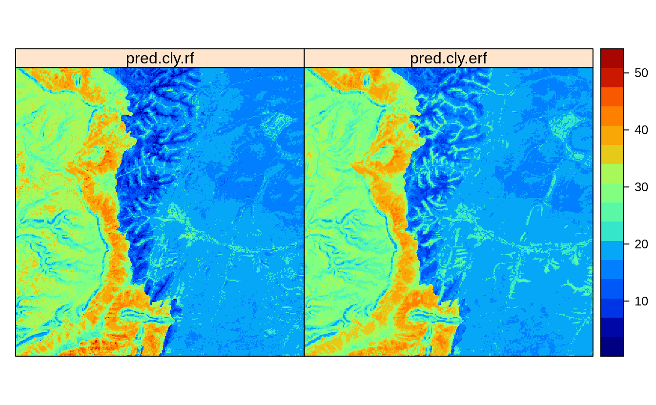
Figure 2.3: Predictions of clay content: (left) ignoring spatial clustering effect on model, (right) after de-clustering of points.
Overall, the difference is small but there is certainly visible difference in predictions.
To the end users we would probably suggest to use pred.cly.erf (predictions produced
using the de-clustered points) map because the other model completely ignores
spatial clustering of points and this could have resulted in bias estimate of the
regression parameters. This solution to producing predictions is fully scalable
and relatively easy to implement, it only requires from user to decide on (1)
size of the block for subsampling, (2) max sampling intensity per block. In practice,
both could be determined by iterations.
2.3 Weighted Machine Learning
Note that the function grid.sample per definition draws points that are relatively
isolated (Fig. 1.3) with higher probability. Hence, a more generic
approach (Strategy #2) from declustering, is to use the case.weights parameter
to instruct ranger to put more emphasis on isolated points / remove impact of
clustered points. This weighted estimation of model parameters is common in regression,
and also in spatial statistics (see e.g. the nlme::gls Generalized Least Square (GLS) function).
Theoretical basis for GLS / weighted regression is that the points that are clustered
might also be spatially correlated, and that means that they would introduce bias in
estimation of the regression parameters. Ideally, regression residuals should be
uncorrelated and uniform, hence a correction is needed that helps ensure these properties.
Weighted Machine Learning where bias in the sampling intensity is incorporated in
the modeling can be implemented in two steps. First, we derive the occurrence
probability (0–1) using the spsample.prob method:
iprob.all <- landmap::spsample.prob(eberg.sp, eberg_spc@predicted[1:4])
#> Deriving kernel density map using sigma 157 ...
#> Deriving inclusion probabilities using MaxLike analysis...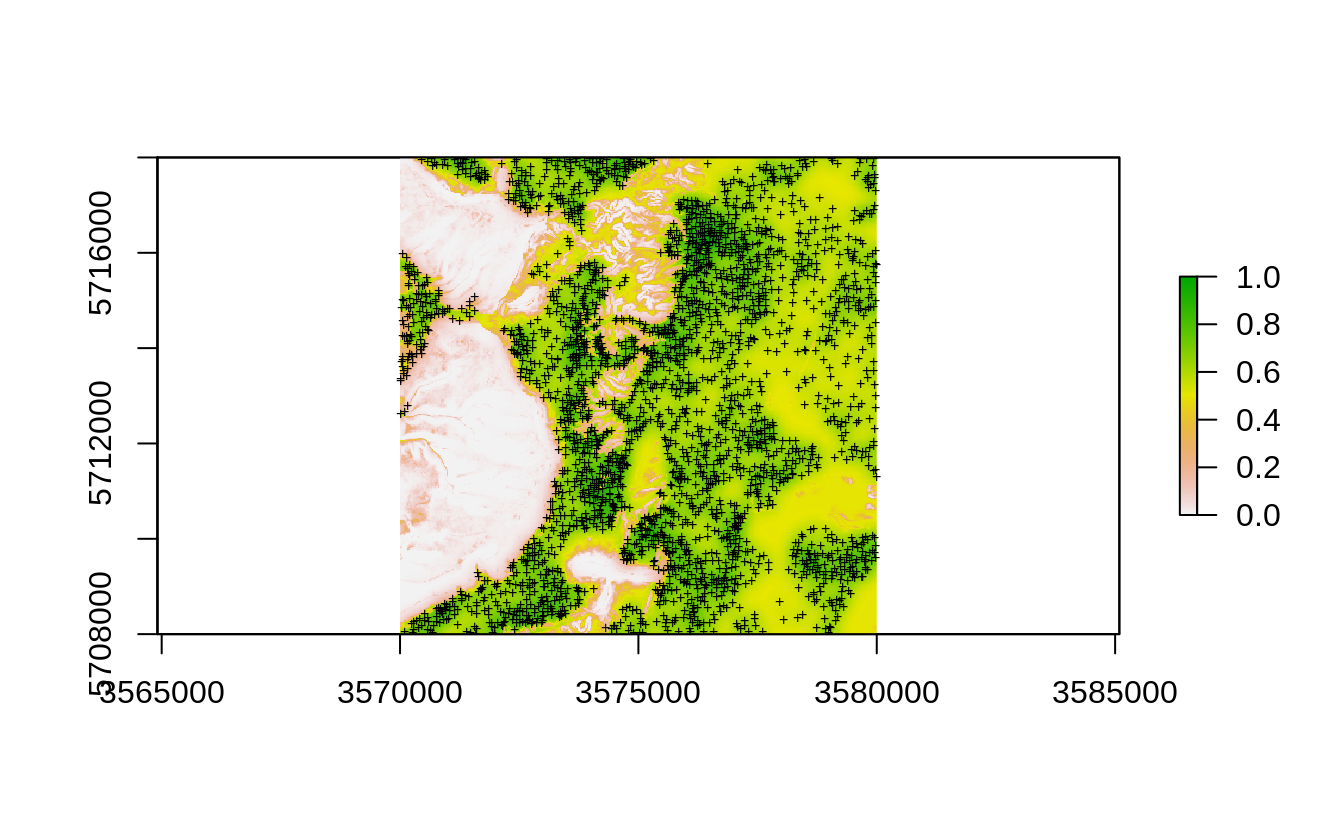
Figure 2.4: Occurrence probability for existing point samples for the Ebergotzen case study derived as an average between the kernel density and maxlike occurrence probabilities.
Second, we fit a model using all points, but this time we set case.weights to be
reversely proportional to probability of occurrence (hence points with lower occurrence
probability get higher weights):
ov.weigths = 1/sp::over(eberg.xy, iprob.all$prob)[]
rf.clyI = ranger::ranger(cly.fm, data=rm.cly, case.weights = ov.weigths[sel.cly,])
Weighted regression is a common technique in statistics and in this case the weights are used to helps reduce clustering effect i.e. give weights to points proportionally to the sampling bias. This method is in principle similar to the nlme::gls Generalized Least Square (GLS) procedure, but with the difference that we do not estimate any spatial autocorrelation structure, but instead incorporate the probability of occurrence to reduce effect of spatial clustering.
2.4 Resampling using Ensemble ML
Another approach to improve generating BUPS from clustered point data is to switch to Ensemble ML i.e. use a multitude of ML methods (so called base-learners), then estimate final predictions using robust resampling and blocking. Ensemble ML has shown to help increase mapping accuracy, but also helps with reducing over-shooting effects due to extrapolation.
One way to reduce effects of point clustering for predictive is to use spatial blocking i.e. to make sure that spatially clustered points are not used both for training and internal validation (Roberts et al., 2017). First, we need to define a spatial grid that we will use as a blocking parameter. We set here arbitrarily size of spatial blocks to 500-m, in practice the block size can be determined more objectively by e.g. analyzing at which distances is clustering reduced:
grd <- sp::GridTopology(cellcentre.offset=eberg_grid25@bbox[,1], cellsize=rep(500,2),
                        cells.dim=c(ceiling(abs(diff(eberg_grid25@bbox[1,])/500))+1,
                        ceiling(abs(diff(eberg_grid25@bbox[2,])/500))+1))
r.sp <- sp::SpatialGridDataFrame(grd, proj4string = eberg_grid25@proj4string,
                    data=data.frame(gid=1:(grd@cells.dim[1] * grd@cells.dim[2])))
id <- sp::over(eberg.xy, r.sp)$gid
#summary(as.factor(id))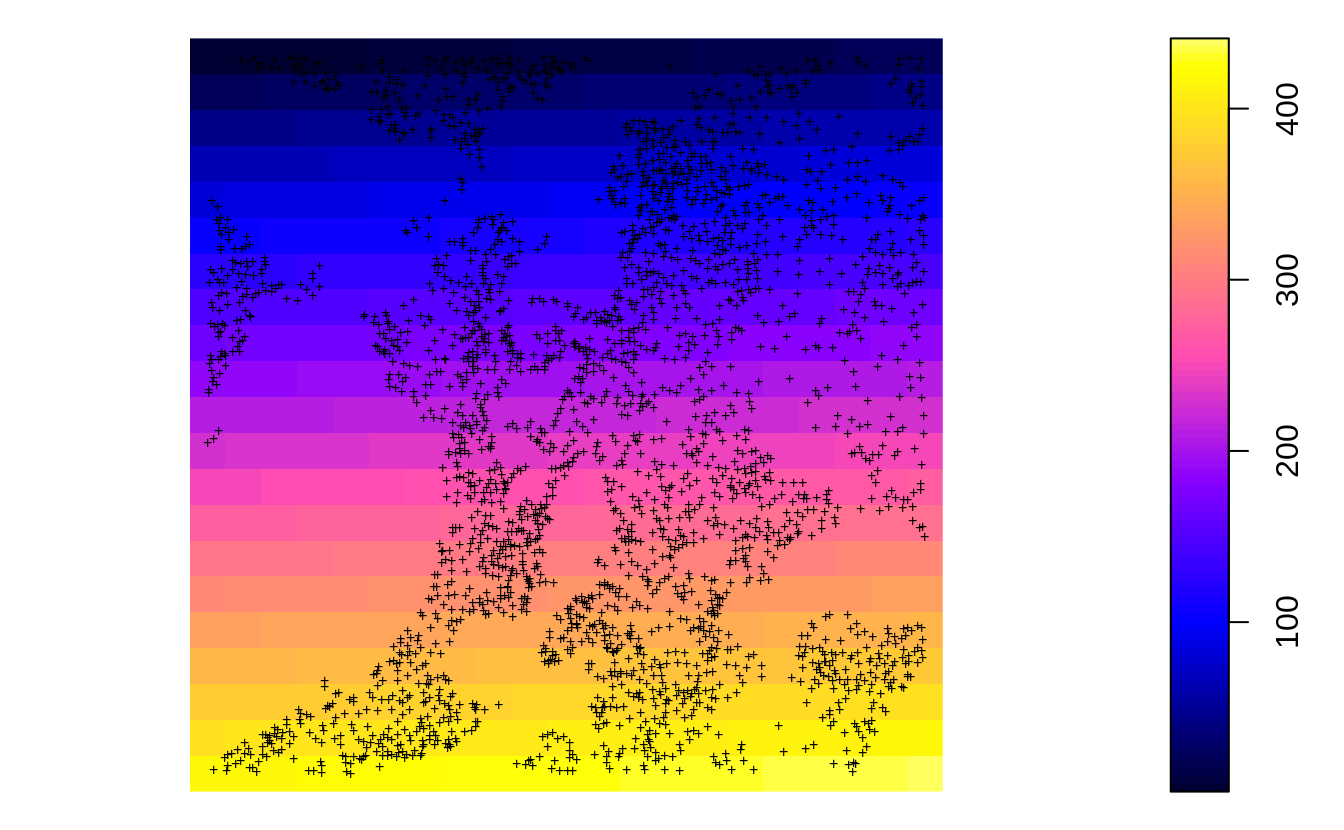
Figure 2.5: 500 m grid for spatial resampling.
This shows that many blocks basically have no training points, and some blocks are densely sampled with e.g. 15–20 points. Next, we can compare models fitted using spatial blocking vs no special settings. First, we fit ensemble ML model using no blocking:
parallelMap::parallelStartSocket(parallel::detectCores())
#> Starting parallelization in mode=socket with cpus=32.
library(mlr)
library(glmnet)
library(Cubist)
lrns <- list(mlr::makeLearner("regr.ranger",
                num.threads = parallel::detectCores(), num.trees=150, importance="impurity"),
             mlr::makeLearner("regr.glm"), mlr::makeLearner("regr.cubist"),
             mlr::makeLearner("regr.cvglmnet"))
tsk0 <- mlr::makeRegrTask(data = rm.cly[,all.vars(cly.fm)], target = "CLYMHT_A")
init0.m <- mlr::makeStackedLearner(lrns, method = "stack.cv",
                                  super.learner = "regr.lm",
                                  resampling=mlr::makeResampleDesc(method = "CV"))
eml0 = train(init0.m, tsk0)
#> Exporting objects to slaves for mode socket: .mlr.slave.options
#> Mapping in parallel: mode = socket; level = mlr.resample; cpus = 32; elements = 10.
#> Exporting objects to slaves for mode socket: .mlr.slave.options
#> Mapping in parallel: mode = socket; level = mlr.resample; cpus = 32; elements = 10.
#> Exporting objects to slaves for mode socket: .mlr.slave.options
#> Mapping in parallel: mode = socket; level = mlr.resample; cpus = 32; elements = 10.
#> Exporting objects to slaves for mode socket: .mlr.slave.options
#> Mapping in parallel: mode = socket; level = mlr.resample; cpus = 32; elements = 10.
summary(eml0$learner.model$super.model$learner.model)
#>
#> Call:
#> stats::lm(formula = f, data = d)
#>
#> Residuals:
#>     Min      1Q  Median      3Q     Max
#> -33.228  -4.005   0.298   3.054  37.818
#>
#> Coefficients:
#>               Estimate Std. Error t value Pr(>|t|)
#> (Intercept)   -0.55143    0.47112  -1.170 0.241906
#> regr.ranger    0.80513    0.05689  14.152  < 2e-16 ***
#> regr.glm       0.24905    0.11067   2.250 0.024502 *
#> regr.cubist    0.13973    0.04208   3.320 0.000911 ***
#> regr.cvglmnet -0.17004    0.11544  -1.473 0.140868
#> ---
#> Signif. codes:  0 '***' 0.001 '**' 0.01 '*' 0.05 '.' 0.1 ' ' 1
#>
#> Residual standard error: 7.339 on 2771 degrees of freedom
#> Multiple R-squared:  0.6041, Adjusted R-squared:  0.6036
#> F-statistic:  1057 on 4 and 2771 DF,  p-value: < 2.2e-16
This shows that ranger i.e. random forest and cubist are the most important
learners and the overall model performance matches the previously fitted model using ranger.
Next, we fit an ensemble ML model with the spatial blocking (500-m):
tsk1 <- mlr::makeRegrTask(data = rm.cly[,all.vars(cly.fm)], target = "CLYMHT_A",
                          blocking = as.factor(id[sel.cly]))
init1.m <- mlr::makeStackedLearner(lrns, method = "stack.cv",
                  super.learner = "regr.lm",
                  resampling=mlr::makeResampleDesc(method = "CV", blocking.cv=TRUE))
eml1 = train(init1.m, tsk1)
#> Exporting objects to slaves for mode socket: .mlr.slave.options
#> Mapping in parallel: mode = socket; level = mlr.resample; cpus = 32; elements = 10.
#> Exporting objects to slaves for mode socket: .mlr.slave.options
#> Mapping in parallel: mode = socket; level = mlr.resample; cpus = 32; elements = 10.
#> Exporting objects to slaves for mode socket: .mlr.slave.options
#> Mapping in parallel: mode = socket; level = mlr.resample; cpus = 32; elements = 10.
#> Exporting objects to slaves for mode socket: .mlr.slave.options
#> Mapping in parallel: mode = socket; level = mlr.resample; cpus = 32; elements = 10.
summary(eml1$learner.model$super.model$learner.model)
#>
#> Call:
#> stats::lm(formula = f, data = d)
#>
#> Residuals:
#>     Min      1Q  Median      3Q     Max
#> -31.676  -4.201   0.443   3.109  40.386
#>
#> Coefficients:
#>               Estimate Std. Error t value Pr(>|t|)
#> (Intercept)   -0.36065    0.48143  -0.749   0.4539
#> regr.ranger    0.63875    0.05688  11.229  < 2e-16 ***
#> regr.glm       0.21547    0.11185   1.926   0.0542 .
#> regr.cubist    0.23915    0.04124   5.800  7.4e-09 ***
#> regr.cvglmnet -0.08255    0.11581  -0.713   0.4760
#> ---
#> Signif. codes:  0 '***' 0.001 '**' 0.01 '*' 0.05 '.' 0.1 ' ' 1
#>
#> Residual standard error: 7.514 on 2771 degrees of freedom
#> Multiple R-squared:  0.5851, Adjusted R-squared:  0.5845
#> F-statistic: 976.9 on 4 and 2771 DF,  p-value: < 2.2e-16
which shows a difference: the RMSE drops for 10–20% and the regr.glm learner is
now also significant. In the previous example, it is possible that the regr.glm model
was possibly shadowed by the fitting power of ranger and Cubist, while after
more strict CV, also more simple models seem to perform with a comparable accuracy.
We can produce predictions using the Ensemble ML model developed with blocking by running:
pred.cly.eml = predict(eml1, newdata=eberg_spc@predicted@data[,eml1$features])
eberg_grid25$pred.cly.eml = pred.cly.eml$data$response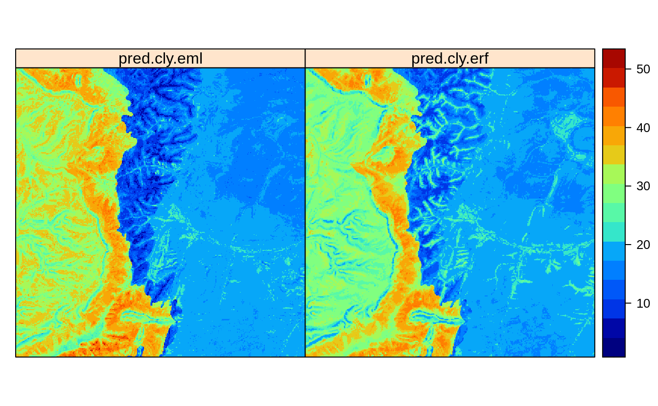
Figure 2.6: Predictions of clay content: (left) Ensemble ML with spatial blocking, (right) after de-clustring of points.
Visual comparison with the predictions produced in previous section, show that
the Ensemble method pred.cly.eml predicts somewhat higher clay content in the
extrapolation area, but also smooths out some higher values in the plains.
Again, if we have to choose we would suggest users to use the map on the left for
two main reasons:
- It is based on multiple base-learners, not only on Random Forest and results
show that both Cubist and glmnet package produce comparable results to RF.
- It is probably more sensible to use the predictions produced by the meta-learner, especially in the extrapolation space.
2.5 Estimating the Area of Applicability
Meyer & Pebesma (2021) have developed a method to estimate so-called “Area of Applicability” using a fitted model and feature space analysis. This method can be used for post-modeling analysis and helps users realize what are the true extrapolation areas and where the predictions are critically poor. The users can then choose to e.g. limit predictions only to combinations of pixels that are NOT too risky (extrapolation).
For the RF model fitted above we can derive AoA using:
library(CAST)
train.df = rm.cly[,all.vars(cly.fm)[-1]]
weight = as.data.frame(mlr::getFeatureImportance(eml1$learner.model$base.models[[1]])$res)
AOA <- CAST::aoa(train=train.df, predictors=eberg_spc@predicted@data[,eml1$features], weight=weight)
This method can be computational so it is probably not recommended for larger datasets. Some example of the Area of Applicability can be found in the CAST package tutorial.
2.6 Estimating per-pixel mapping accuracy
Using the Ensemble Model we can also estimate the mapping accuracy per pixel i.e. by deriving the Mean Square Prediction Error (MSPE). The forestError package currently provides a “Unified Framework for Random Forest Prediction Error Estimation” (Lu & Hardin, 2021) and is probably the most worked-out procedure for deriving prediction errors and estimating potential bias. This requires two steps, (1) first, we need to fit an additional quantile Regression RF model (using the four base learners from the previous section), (2) second, we can then estimate complete error statistics per pixel using the quantForestError function.
Because derivation of prediction errors per pixel can often be computational (even at the order of magnitude more computational than predictions), it is important to use a method that is computationally efficient and precise enough. In the landmap package the uncertainty is derived using base learners instead of using ALL raster layers which could be hundreds. This approach of using (few) base learners instead of (many) original covariates helps compress the complexity of model and significantly speed-up computing. The base learners can be accessed from the mlr object:
eml.t = eml1$learner.model$super.model$learner.model$terms
paste(eml.t)
#> [1] "~"
#> [2] "CLYMHT_A"
#> [3] "regr.ranger + regr.glm + regr.cubist + regr.cvglmnet"
eml.m = eml1$learner.model$super.model$learner.model$model
We use the spatially resampled base-learners to fit (an independent) quantile RF:
eml.qr <- ranger::ranger(eml.t, eml.m, num.trees=85, importance="impurity",
                         quantreg=TRUE, keep.inbag = TRUE)
#eml.qr
Next, we can use the forestError package to derive prediction errors by:
library(forestError)
quantiles = c((1-.682)/2, 1-(1-.682)/2)
n.cores = parallel::detectCores()
out.c <- as.data.frame(mlr::getStackedBaseLearnerPredictions(eml1,
          newdata=eberg_spc@predicted@data[,eml1$features]))
pred.q = forestError::quantForestError(eml.qr,
                    X.train = eml.m[,all.vars(eml.t)[-1]],
                    X.test = out.c,
                    Y.train = eml.m[,all.vars(eml.t)[1]],
                    alpha = (1-(quantiles[2]-quantiles[1])), n.cores=n.cores)
We could have also subset e.g. 10% of the input points and keep them ONLY for
estimating the prediction errors using the quantForestError, which is also
recommended by the authors of the forestError package. In practice, because
base learners have been fitted using 5-fold Cross-Validation with blocking,
they are already out-of-bag samples hence taking out extra OOB samples is
probably not required, but you can also test this with your own data.
The quantForestError function runs a complete uncertainty assessment and
includes both MSPE, bias and upper and lower confidence intervals:
str(pred.q)
#> List of 3
#>  $ estimates:'data.frame':   160000 obs. of  5 variables:
#>   ..$ pred       : num [1:160000] 35.2 37.5 31.7 36 35.9 ...
#>   ..$ mspe       : num [1:160000] 138.1 104.1 82.7 90.9 76.2 ...
#>   ..$ bias       : num [1:160000] -1.77 -1.22 -1.13 -1.18 -1.45 ...
#>   ..$ lower_0.318: num [1:160000] 23.5 27.8 21.5 29.6 29.5 ...
#>   ..$ upper_0.318: num [1:160000] 52.7 47.7 40.2 47.7 42.3 ...
#>  $ perror   :function (q, xs = 1:n.test)
#>  $ qerror   :function (p, xs = 1:n.test)
In this case, for the lower and upper confidence intervals we use 1-standard deviation probability which is about 2/3 probability and hence the lower value is 0.159 and upper 0.841. The RMSPE should match the half of the difference between the lower and upper interval in this case, although there will be difference in exact numbers.
The mean RMSPE for the whole study area (mean of all pixels) should be as expected somewhat higher than the RMSE we get from model fitting:
This is because we are also extrapolating in the large part of the area. The map in Fig. 2.7 correctly depicts the extrapolation areas as having much higher RMSPE (compare with Fig. 2.4):
eberg_grid25$rmspe.cly.eml = sqrt(pred.q$estimates$mspe)
plot(raster(eberg_grid25[c("rmspe.cly.eml")]), col=SAGA_pal[[16]])
points(eberg.sp, pch="+", cex=.6)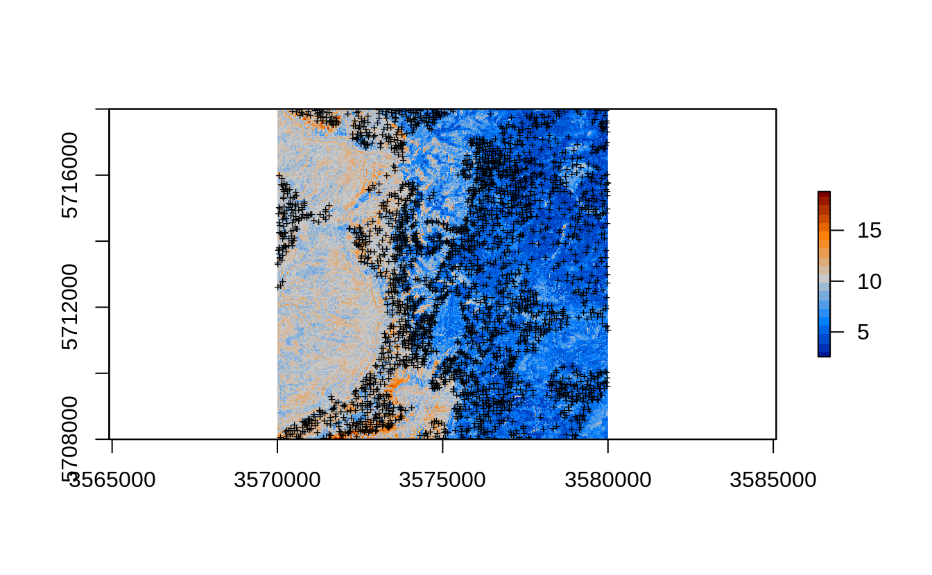
Figure 2.7: Prediction errors for the clay content based on the forestError package and Ensemble ML.
In the previous examples we have shown that the actual samples from the Ebergotzen dataset are actually clustered and cover only agricultural land. Can we still use these samples to estimate the mapping accuracy for the whole area? The answer is yes, but we need to be aware that our estimate might be biased (usually over-optimistic) and we need to do our best to reduce the over-fitting effects by implementing some of the strategies above e.g.: assign different weights to training points, and/or implement blocking settings.
Assuming that forest soils are possibly very different from agricultural soils, once we collect new sampling in the forest part of the study area we might discovering that the actual mapping accuracy we estimated for the whole study area using only agricultural soil samples is significantly lower than what we have estimated in Fig. 2.7.
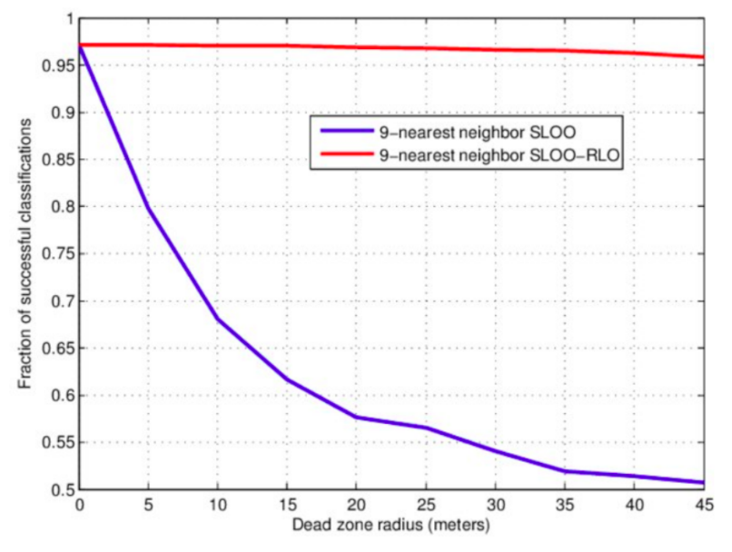
Figure 2.8: Example of effects of the size of the spatial blocking (buffer) on mapping accuracy.
Fig. 2.8 shows the usual effect of spatial blocking (for varying buffer size) on the Cross-Validation accuracy (Pohjankukka, Pahikkala, Nevalainen, & Heikkonen, 2017). Note that the accuracy tends to stabilize at some distance, although too strict blocking can also lead to over-pessimistic estimates of accuracy hence bias in predictions (@ Wadoux, Heuvelink, de Bruin, & Brus, 2021). In the Ebergotzen case, prediction error could be over-pessimistic although the block size is relatively small considering the size of the study area. On the other hand, if the training points are clustered, blocking becomes important because otherwise the estimate of error and choice of model parameters could get over-optimistic (Lovelace, Nowosad, & Muenchow, 2019; Meyer, Reudenbach, Hengl, Katurji, & Nauss, 2018). If in doubt of whether to produce over-optimistic or over-pessimistic estimates of uncertainty, it is of course ideal to avoid both, but if necessary consider that somewhat over-pessimistic estimate of accuracy could be slightly more on a safe side (Roberts et al., 2017).
2.7 Testing mapping accuracy using resampling and blocking
We can switch to the Edgeroi dataset (Malone, McBratney, Minasny, & Laslett, 2009) that is originally based on designed sampling and as such is more interesting for assessing effects of various blocking strategies on overall mapping accuracy. We can load the dataset and prepare a regression matrix by using (Hengl & MacMillan, 2019):
data(edgeroi)
edgeroi.sp <- edgeroi$sites
coordinates(edgeroi.sp) <- ~ LONGDA94 + LATGDA94
proj4string(edgeroi.sp) <- CRS("+proj=longlat +ellps=GRS80 +towgs84=0,0,0,0,0,0,0 +no_defs")
edgeroi.sp <- spTransform(edgeroi.sp, CRS("+init=epsg:28355"))
length(edgeroi.sp)
#> [1] 359
h2 <- hor2xyd(edgeroi$horizons)
edgeroi.grids.100m = readRDS("./extdata/edgeroi.grids.100m.rds")
edgeroi.grids = landmap::spc(edgeroi.grids.100m[-1])
#> Converting covariates to principal components...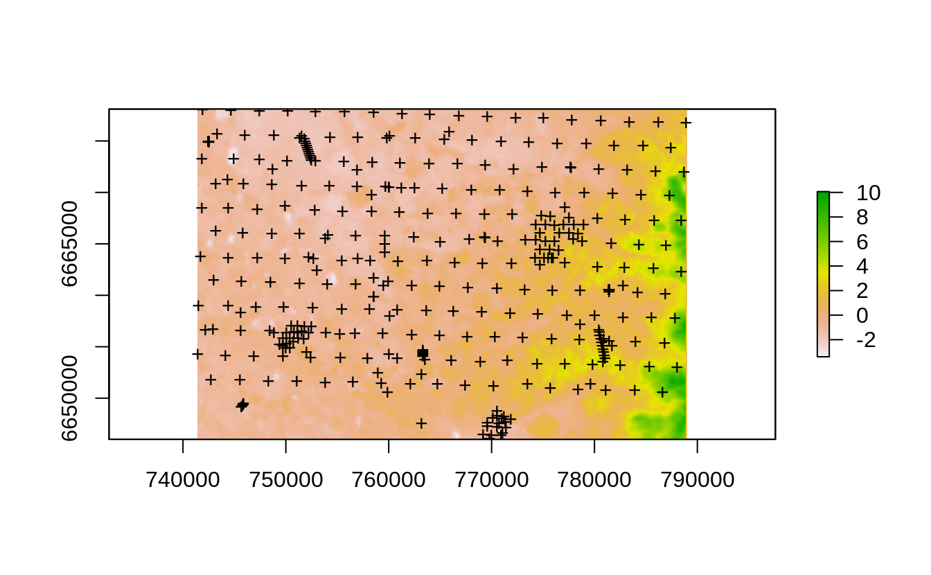
Figure 2.9: The Edgeroi dataset consisting of 359 soil profiles.
The dataset documentation indicates that from a total of 359 profiles, 210 soil profiles were sampled on a systematic, equilateral triangular grid with a spacing of 2.8 km between sites; the further 131 soil profiles are distributed more irregularly or on transects (Malone, McBratney, Minasny, & Laslett, 2009). This is hence a hybrid sampling design but in general satisfying IID, and hence any subsample of these points should give an unbiased estimate of the mapping accuracy. We first prepare a regression matrix that includes all covariates, location IDs and we also add a spatial grid of 500-m size:
grdE <- sp::GridTopology(cellcentre.offset=edgeroi.grids.100m@bbox[,1], cellsize=rep(500,2),
                        cells.dim=c(ceiling(abs(diff(edgeroi.grids.100m@bbox[1,])/500))+1,
                        ceiling(abs(diff(edgeroi.grids.100m@bbox[2,])/500))+1))
rE.sp <- sp::SpatialGridDataFrame(grdE, proj4string = edgeroi.grids.100m@proj4string,
                    data=data.frame(gid=1:(grdE@cells.dim[1] * grdE@cells.dim[2])))
ovF <- sp::over(edgeroi.sp, edgeroi.grids@predicted)
ovF$SOURCEID <- edgeroi.sp$SOURCEID
ovF$gid <- sp::over(edgeroi.sp, rE.sp)$gid
ovF$x = edgeroi.sp@coords[,1]
ovF$y = edgeroi.sp@coords[,2]
rmF <- plyr::join_all(dfs = list(edgeroi$sites, h2, ovF))
#> Joining by: SOURCEID
#> Joining by: SOURCEID
This produces a regression matrix with unique IDs of profiles SOURCEID, spatial
block IDs (gid) and all target and covariate layers.
We can now fit a model to predict soil organic carbon content (in g/kg) in 3D:
rmF$log.ORCDRC = log1p(rmF$ORCDRC)
formulaStringPF <- as.formula(paste0("log.ORCDRC ~ DEPTH + ", paste0("PC", 1:10, collapse = "+")))
rmPF <- rmF[complete.cases(rmF[,all.vars(formulaStringPF)]),]
#str(rmPF[,all.vars(formulaStringPF)])
We first fit a model distribution of soil organic carbon ignoring any spatial clustering, overlap in 3rd dimension (soil depth) or similar:
soc.rf = ranger(formulaStringPF, rmPF)
soc.rf
#> Ranger result
#>
#> Call:
#>  ranger(formulaStringPF, rmPF)
#>
#> Type:                             Regression
#> Number of trees:                  500
#> Sample size:                      5001
#> Number of independent variables:  11
#> Mtry:                             3
#> Target node size:                 5
#> Variable importance mode:         none
#> Splitrule:                        variance
#> OOB prediction error (MSE):       0.1116369
#> R squared (OOB):                  0.8166682
If we compare this model with an Ensemble ML where whole blocks i.e. including also whole soil profiles are taken out from modeling:
SL.library2 = c("regr.ranger", "regr.glm", "regr.cvglmnet", "regr.xgboost", "regr.ksvm")
lrnsE <- lapply(SL.library2, mlr::makeLearner)
tskE <- mlr::makeRegrTask(data = rmPF[,all.vars(formulaStringPF)], target="log.ORCDRC",
                          blocking = as.factor(rmPF$gid))
initE.m <- mlr::makeStackedLearner(lrnsE, method = "stack.cv",
                  super.learner = "regr.lm",
                  resampling=mlr::makeResampleDesc(method = "CV", blocking.cv=TRUE))
emlE = train(initE.m, tskE)
#> Exporting objects to slaves for mode socket: .mlr.slave.options
#> Mapping in parallel: mode = socket; level = mlr.resample; cpus = 32; elements = 10.
#> Exporting objects to slaves for mode socket: .mlr.slave.options
#> Mapping in parallel: mode = socket; level = mlr.resample; cpus = 32; elements = 10.
#> Exporting objects to slaves for mode socket: .mlr.slave.options
#> Mapping in parallel: mode = socket; level = mlr.resample; cpus = 32; elements = 10.
#> Exporting objects to slaves for mode socket: .mlr.slave.options
#> Mapping in parallel: mode = socket; level = mlr.resample; cpus = 32; elements = 10.
#> [10:39:09] WARNING: amalgamation/../src/objective/regression_obj.cu:170: reg:linear is now deprecated in favor of reg:squarederror.
#> Exporting objects to slaves for mode socket: .mlr.slave.options
#> Mapping in parallel: mode = socket; level = mlr.resample; cpus = 32; elements = 10.
summary(emlE$learner.model$super.model$learner.model)
#>
#> Call:
#> stats::lm(formula = f, data = d)
#>
#> Residuals:
#>     Min      1Q  Median      3Q     Max
#> -2.1642 -0.2550 -0.0232  0.2376  3.1830
#>
#> Coefficients:
#>               Estimate Std. Error t value Pr(>|t|)
#> (Intercept)   -0.17386    0.03557  -4.887 1.05e-06 ***
#> regr.ranger    0.83042    0.04432  18.736  < 2e-16 ***
#> regr.glm       0.42906    0.07066   6.072 1.36e-09 ***
#> regr.cvglmnet -0.37021    0.07626  -4.855 1.24e-06 ***
#> regr.xgboost   0.20284    0.09370   2.165   0.0305 *
#> regr.ksvm      0.12077    0.02840   4.253 2.15e-05 ***
#> ---
#> Signif. codes:  0 '***' 0.001 '**' 0.01 '*' 0.05 '.' 0.1 ' ' 1
#>
#> Residual standard error: 0.449 on 4995 degrees of freedom
#> Multiple R-squared:  0.6693, Adjusted R-squared:  0.6689
#> F-statistic:  2022 on 5 and 4995 DF,  p-value: < 2.2e-16
Notice a large difference in the model accuracy with R-square dropping from about 0.82 to 0.65. How can we check which of the two models is more accurate / which shows a more realistic mapping accuracy? We can again generate pseudo-grid samples e.g. 10 subsets where in each subset we make sure that the points are at least 3.5-km apart and are taken selected randomly:
subE.lst = lapply(1:10, function(i){landmap::sample.grid(edgeroi.sp, c(3.5e3, 3.5e3), n=1)})
lE1 <- list("sp.points", subE.lst[[1]]$subset, pch="+", col="black")
spplot(subE.lst[[1]]$grid, scales=list(draw=TRUE),
   col.regions="grey", sp.layout=list(lE1), colorkey=FALSE)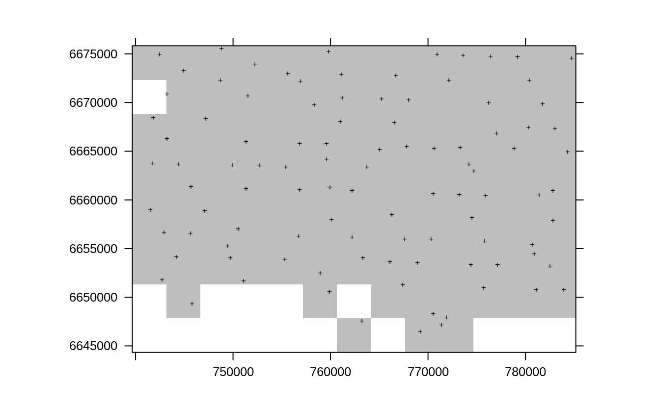
Figure 2.10: Resampling original points using sample.grid function for the Edgeroi dataset.
So in any random pseudo-grid subset we take out about 100 profiles from 359 and keep for validation only. We can next repeatedly fit models using the two approaches and derive prediction errors. First, for simple model ignoring any spatial clustering / soil profile locations:
rf.soc.lst = lapply(1:length(subE.lst), function(i){
        sel <- !rmPF$SOURCEID %in% subE.lst[[i]]$subset$SOURCEID;
        y <- ranger::ranger(formulaStringPF, rmPF[sel,]);
        out <- data.frame(meas=rmPF[!sel,"log.ORCDRC"], pred=predict(y, rmPF[!sel,])$predictions);
        return(out)
      }
)
rf.cv = do.call(rbind, rf.soc.lst)
Metrics::rmse(rf.cv$meas, rf.cv$pred)
#> [1] 0.4343792
This gives an RMSPE of 0.44, which is higher than what is reported by the OOB for RF without blocking. The accuracy plot shows that the Concordance Correlation Coefficient (CCC) is about 0.79 (corresponding to a R-square of about 0.62 and thus significantly less than what is reported by ranger):
t.b = quantile(log1p(rmPF$ORCDRC), c(0.001, 0.01, 0.999), na.rm=TRUE)
plot_hexbin(varn="SOC_RF", breaks=c(t.b[1], seq(t.b[2], t.b[3], length=25)),
      meas=rf.cv$meas, pred=rf.cv$pred, main="SOC [RF]")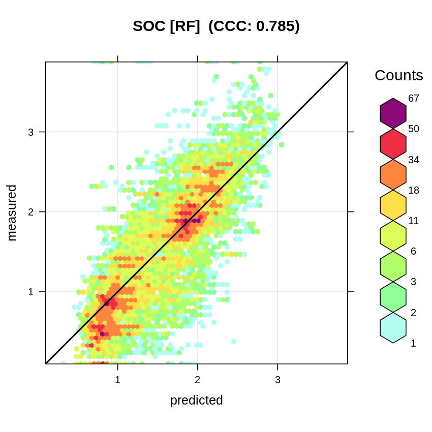
Figure 2.11: Accuracy plot for soil organic carbon fitted using RF.
We repeat the same process of re-fitting the model using Ensemble ML with spatial blocking:
eml.soc.lst = lapply(1:length(subE.lst), function(i){
        sel <- !rmPF$SOURCEID %in% subE.lst[[i]]$subset$SOURCEID;
        x <- mlr::makeRegrTask(data = rmPF[sel,all.vars(formulaStringPF)],
                  target="log.ORCDRC", blocking = as.factor(rmPF$gid[sel]));
        y <- train(initE.m, x)
        out <- data.frame(meas=rmPF[!sel,"log.ORCDRC"], pred=predict(y, newdata=rmPF[!sel, y$features])$data$response);
        return(out)
      }
)
eml.cv = do.call(rbind, eml.soc.lst)
Metrics::rmse(eml.cv$meas, eml.cv$pred)
plot_hexbin(varn="SOC_EML", breaks=c(t.b[1], seq(t.b[2], t.b[3], length=25)),
      meas=eml.cv$meas, pred=eml.cv$pred, main="SOC [EML]")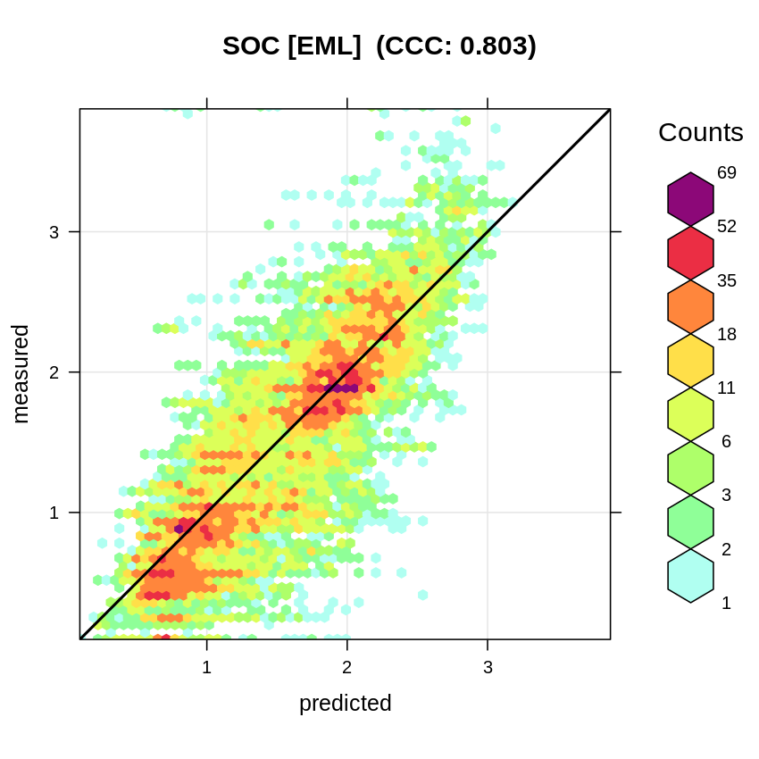
Figure 2.12: Accuracy plot for soil organic carbon fitted using Ensemble Machine Learning with spatial blocking.
So in summary, independent validation using pseudo-probability samples indicates
that the Ensemble ML produces more accurate predictions (in this case only slightly
better) and the RMSE estimated by the meta-learner the Ensemble ML approach is more
realistic (Residual standard error: 0.45). This clearly demonstrates that spatial
blocking is important to (a) prevent from over-fitting, (b) produce a more realistic
estimate of the uncertainty / mapping accuracy. Ensemble ML comes at costs of
at the order of magnitude higher computing costs however.
We can again plot the predictions produced by two methods next to each other:
newdata = edgeroi.grids@predicted@data[,paste0("PC", 1:10)]
newdata$DEPTH = 5
edgeroi.grids.100m$rf_soc_5cm = predict(soc.rf, newdata)$predictions
edgeroi.grids.100m$eml_soc_5cm = predict(emlE, newdata=newdata[,emlE$features])$data$response
l.pnts <- list("sp.points", edgeroi.sp, pch="+", col="black")
spplot(edgeroi.grids.100m[c("rf_soc_5cm", "eml_soc_5cm")],
       sp.layout = list(l.pnts), col.regions=SAGA_pal[[1]])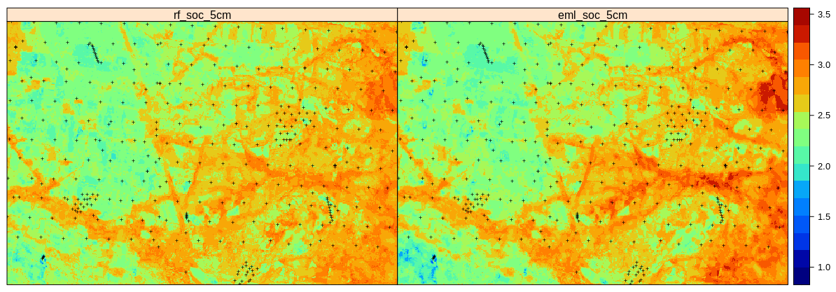
Figure 2.13: Predictions of soil organic carbon (in log-scale) based on Random Forest (RF) and Ensemble ML (EML).
Which shows that the Ensemble ML seems to predict significantly higher SOC in the hillands (right part of the study area), so again significant difference in predictions between the two models. Even though the Ensemble ML with spatial blocking is only slightly better in accuracy (RMSE based on 10-times out-of-bag declustered validation points), these results confirm that it helps produce a more realistic map of RMSPE. This matches the result of Roberts et al. (2017) and Meyer, Reudenbach, Hengl, Katurji, & Nauss (2018) who suggest that block cross-validation is nearly universally more appropriate than random cross-validation if the goal is predicting to new data or predictor space, or for selecting causal predictors.
We can also map the prediction errors:
emlE.t = emlE$learner.model$super.model$learner.model$terms
paste(emlE.t)
#> [1] "~"
#> [2] "log.ORCDRC"
#> [3] "regr.ranger + regr.glm + regr.cvglmnet + regr.xgboost + regr.ksvm"
emlE.m = emlE$learner.model$super.model$learner.model$model
emlE.qr <- ranger::ranger(emlE.t, emlE.m, num.trees=85, importance="impurity",
                         quantreg=TRUE, keep.inbag = TRUE)
outE.c <- as.data.frame(mlr::getStackedBaseLearnerPredictions(emlE,
                                      newdata=newdata[,emlE$features]))
predE.q = forestError::quantForestError(emlE.qr,
                    X.train = emlE.m[,all.vars(emlE.t)[-1]],
                    X.test = outE.c,
                    Y.train = emlE.m[,all.vars(emlE.t)[1]],
                    alpha = (1-(quantiles[2]-quantiles[1])), n.cores=n.cores)
Which again shows where could be the main extrapolation problems i.e. where multiple base learners perform poorly:
edgeroi.grids.100m$rmspe.soc.eml = sqrt(predE.q$estimates$mspe)
plot(raster(edgeroi.grids.100m[c("rmspe.soc.eml")]), col=SAGA_pal[[16]])
points(edgeroi.sp, pch="+", cex=.8)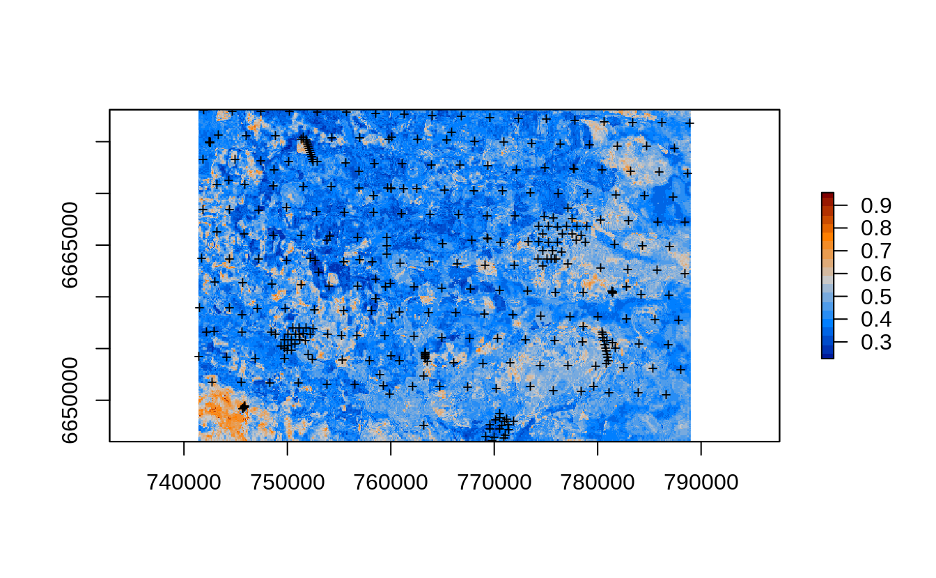
Figure 2.14: Prediction errors for the soil organic carbon content based on the forestError package and Ensemble ML.
rgdal::writeGDAL(edgeroi.grids.100m[c("rmspe.soc.eml")],
                 "./output/edgeroi_soc_rmspe.tif",
                 options=c("COMPRESS=DEFLATE"))
The overall mapping accuracy for Edgeroi based on the mean prediction error is thus:
which in general matches what we get through repeated validation using pseudo-SRS subsampling.
From this experiment we can conclude that the mapping accuracy estimated using ranger and out-of-bag samples and ignoring locations of profiles was probably over-optimistic and hence ranger has possibly over-fitted the target variable. This is in fact common problem observed with many 3D predictive soil mapping models where soil profiles basically have ALL the same values of covariates and Random Forest thus easier predicts values due to overlap in covariate data. For a discussion on why is thus important to run internal training and Cross-Validation using spatial blocking refer also to C. Gasch et al. (2015) and Meyer, Reudenbach, Hengl, Katurji, & Nauss (2018).
parallelMap::parallelStop()
#> Stopped parallelization. All cleaned up.