3.1 Case study: Cookfarm dataset

We next look at the Cookfarm dataset, which is available via the landmap package and described in detail in C. K. Gasch et al. (2015):

library(landmap)
#?landmap::cookfarm
data("cookfarm")

This dataset contains spatio-temporal (3D+T) measurements of three soil properties and a number of spatial and temporal regression covariates. In this example multiple covariates are used to fit a spatiotemporal model to predict soil moisture, soil temperature and electrical conductivity in 3D+T (hence 2 extra dimension beyond spatial dimensions i.e. a 2D model).

We can load the prediction locations and regression-matrix from:

library(rgdal)
library(ranger)
cookfarm.rm = readRDS('extdata/cookfarm_st.rds')
cookfarm.grid = readRDS('extdata/cookfarm_grid10m.rds')

We are specifically interested in modeling soil moisture (VW) as a function of soil depth (altitude), elevation (DEM), Topographic Wetness Index (TWI), Normalized Difference Red Edge Index (NDRE.M), Normalized Difference Red Edge Index (NDRE.sd), Cumulative precipitation in mm (Precip_cum), Maximum measured temperature (MaxT_wrcc), Minimum measured temperature (MinT_wrcc) and the transformed cumulative day (cdayt):

fm <- VW ~ altitude+DEM+TWI+NDRE.M+NDRE.Sd+Precip_cum+MaxT_wrcc+MinT_wrcc+cdayt

We can use the ranger package to fit a random forest model:

m.vw = ranger(fm, cookfarm.rm, num.trees = 100)
m.vw
#> Ranger result
#> 
#> Call:
#>  ranger(fm, cookfarm.rm, num.trees = 100) 
#> 
#> Type:                             Regression 
#> Number of trees:                  100 
#> Sample size:                      107851 
#> Number of independent variables:  9 
#> Mtry:                             3 
#> Target node size:                 5 
#> Variable importance mode:         none 
#> Splitrule:                        variance 
#> OOB prediction error (MSE):       0.0009826038 
#> R squared (OOB):                  0.8479968

which shows that a significant model can be fitting using this data with R-square about 0.85. The accuracy plot shows that the Concordance Correlation Coefficient (CCC) is high:

vw.b = quantile(cookfarm.rm$VW, c(0.001, 0.01, 0.999), na.rm=TRUE)
plot_hexbin(varn="VW_RF", breaks=c(vw.b[1], seq(vw.b[2], vw.b[3], length=25)), 
      meas=cookfarm.rm$VW, pred=m.vw$predictions, main="VW [RF]")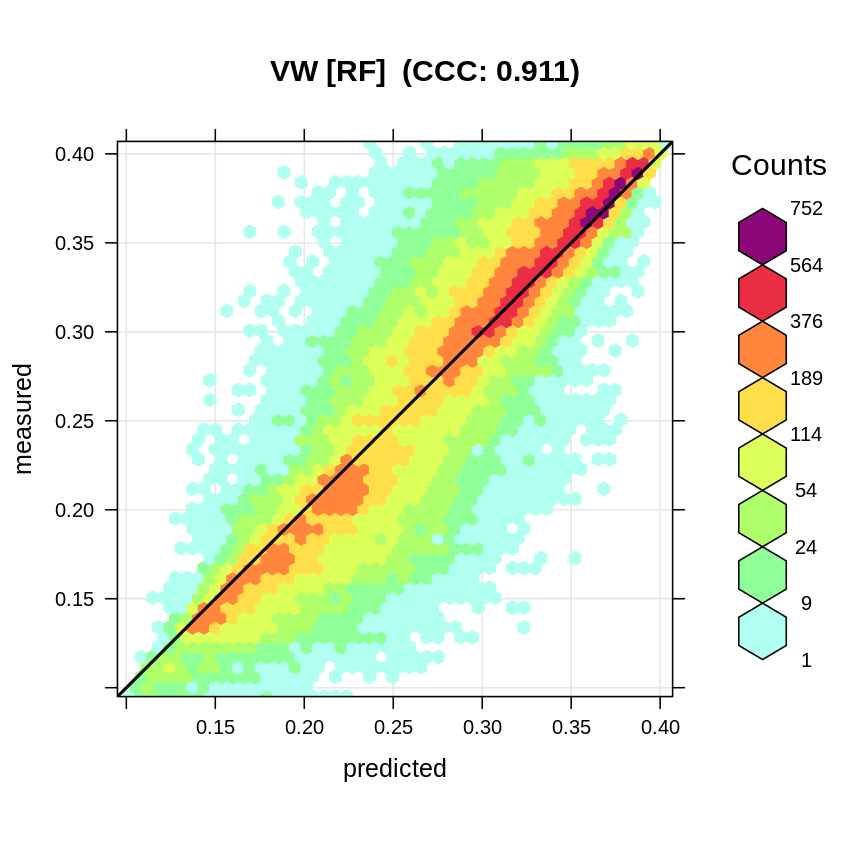

Figure 3.1: Accuracy plot for soil moisture content fitted using RF.

This model, however, as shown in C. K. Gasch et al. (2015), ignores the fact that many VW measurements have exactly the same location (monitoring station with four depths), hence ranger over-fits data and gives unrealistic R-square. We can instead fit an Ensemble ML model, but we will also use a blocking parameter that should protect from over-fitting: the unique code of the station (SOURCEID). This means that complete stations will be either used for training or for validation. This satisfies the requirement of Roberts et al. (2017) for predicting to new data or predictor space by blocking clustered or overlapping measurements.

We use the same procedure in mlr as in the previous example:

library(mlr)
SL.lst = c("regr.ranger", "regr.gamboost", "regr.cvglmnet")
lrns.st <- lapply(SL.lst, mlr::makeLearner)
## subset to 5% to speed up computing
subs <- runif(nrow(cookfarm.rm))<.05
tsk.st <- mlr::makeRegrTask(data = cookfarm.rm[subs, all.vars(fm)], target = "VW", 
                            blocking = as.factor(cookfarm.rm$SOURCEID)[subs])
tsk.st
#> Supervised task: cookfarm.rm[subs, all.vars(fm)]
#> Type: regr
#> Target: VW
#> Observations: 5321
#> Features:
#>    numerics     factors     ordered functionals 
#>           9           0           0           0 
#> Missings: FALSE
#> Has weights: FALSE
#> Has blocking: TRUE
#> Has coordinates: FALSE

The resulting model again used simple linear regression for stacking various learners:

#> Starting parallelization in mode=socket with cpus=32.
#> Exporting objects to slaves for mode socket: .mlr.slave.options
#> Mapping in parallel: mode = socket; level = mlr.resample; cpus = 32; elements = 10.
#> Exporting objects to slaves for mode socket: .mlr.slave.options
#> Mapping in parallel: mode = socket; level = mlr.resample; cpus = 32; elements = 10.
#> Loading required package: mboost
#> Loading required package: parallel
#> Loading required package: stabs
#> 
#> Attaching package: 'stabs'
#> The following object is masked from 'package:mlr':
#> 
#>     subsample
#> The following object is masked from 'package:spatstat.core':
#> 
#>     parameters
#> This is mboost 2.9-2. See 'package?mboost' and 'news(package  = "mboost")'
#> for a complete list of changes.
#> 
#> Attaching package: 'mboost'
#> The following object is masked from 'package:glmnet':
#> 
#>     Cindex
#> The following object is masked from 'package:spatstat.core':
#> 
#>     Poisson
#> The following objects are masked from 'package:raster':
#> 
#>     cv, extract
#> Exporting objects to slaves for mode socket: .mlr.slave.options
#> Mapping in parallel: mode = socket; level = mlr.resample; cpus = 32; elements = 10.
#> Stopped parallelization. All cleaned up.

Note that here we can use full-parallelisation to speed up computing by using the parallelMap package. This resulting EML model now shows a more realistic R-square / RMSE:

summary(eml.VW$learner.model$super.model$learner.model)
#> 
#> Call:
#> stats::lm(formula = f, data = d)
#> 
#> Residuals:
#>       Min        1Q    Median        3Q       Max 
#> -0.188277 -0.044502  0.003824  0.044429  0.177609 
#> 
#> Coefficients:
#>                Estimate Std. Error t value Pr(>|t|)    
#> (Intercept)    0.044985   0.009034   4.979 6.58e-07 ***
#> regr.ranger    1.002421   0.029440  34.050  < 2e-16 ***
#> regr.gamboost -0.664149   0.071813  -9.248  < 2e-16 ***
#> regr.cvglmnet  0.510689   0.052930   9.648  < 2e-16 ***
#> ---
#> Signif. codes:  0 '***' 0.001 '**' 0.01 '*' 0.05 '.' 0.1 ' ' 1
#> 
#> Residual standard error: 0.06262 on 5317 degrees of freedom
#> Multiple R-squared:  0.3914, Adjusted R-squared:  0.3911 
#> F-statistic:  1140 on 3 and 5317 DF,  p-value: < 2.2e-16

The accuracy plot also shows the CCC to be almost 40% smaller than if no blocking is used:

plot_hexbin(varn="VW_EML", breaks=c(vw.b[1], seq(vw.b[2], vw.b[3], length=25)), 
      meas=eml.VW$learner.model$super.model$learner.model$model$VW, 
      pred=eml.VW$learner.model$super.model$learner.model$fitted.values, 
      main="VW [EML]")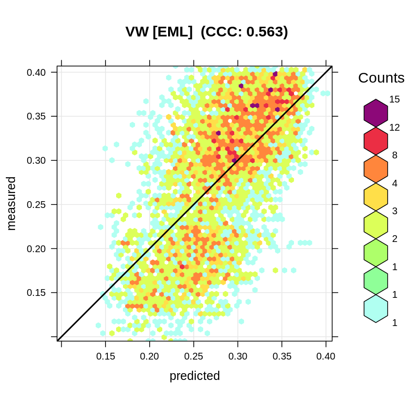

Figure 3.2: Accuracy plot for soil moisture content fitted using Ensemble ML with blocking (taking complete stations out).

The Ensemble ML is now a 3D+T model of VW, which means that we can use it to predict values of VW at any new x,y,d,t location. To make prediction for a specific spacetime slice we use:

cookfarm$weather$Precip_cum <- ave(cookfarm$weather$Precip_wrcc,
                                   rev(cumsum(rev(cookfarm$weather$Precip_wrcc)==0)), FUN=cumsum)
date = as.Date("2012-07-30")
cday = floor(unclass(date)/86400-.5)
cdayt = cos((cday-min(cookfarm.rm$cday))*pi/180)
depth = -0.3
new.st <- data.frame(cookfarm.grid)
new.st$Date = date
new.st$cdayt = cdayt
new.st$altitude = depth
new.st = plyr::join(new.st, cookfarm$weather, type="left")
#> Joining by: Date
## predict:
pr.df = predict(eml.VW, newdata = new.st[,all.vars(fm)[-1]])
#> Warning in bsplines(mf[[i]], knots = args$knots[[i]]$knots, boundary.knots =
#> args$knots[[i]]$boundary.knots, : Some 'x' values are beyond 'boundary.knots';
#> Linear extrapolation used.

#> Warning in bsplines(mf[[i]], knots = args$knots[[i]]$knots, boundary.knots =
#> args$knots[[i]]$boundary.knots, : Some 'x' values are beyond 'boundary.knots';
#> Linear extrapolation used.

#> Warning in bsplines(mf[[i]], knots = args$knots[[i]]$knots, boundary.knots =
#> args$knots[[i]]$boundary.knots, : Some 'x' values are beyond 'boundary.knots';
#> Linear extrapolation used.

#> Warning in bsplines(mf[[i]], knots = args$knots[[i]]$knots, boundary.knots =
#> args$knots[[i]]$boundary.knots, : Some 'x' values are beyond 'boundary.knots';
#> Linear extrapolation used.

To plot prediction together with locations of training points we can use:

cookfarm.grid$pr.VW = pr.df$data$response
plot(raster::raster(cookfarm.grid["pr.VW"]), col=rev(bpy.colors()),
     main="Predicted VW for 2012-07-30 and depth -0.3 m", axes=FALSE, box=FALSE)
points(cookfarm$profiles[,c("Easting","Northing")], pch="+")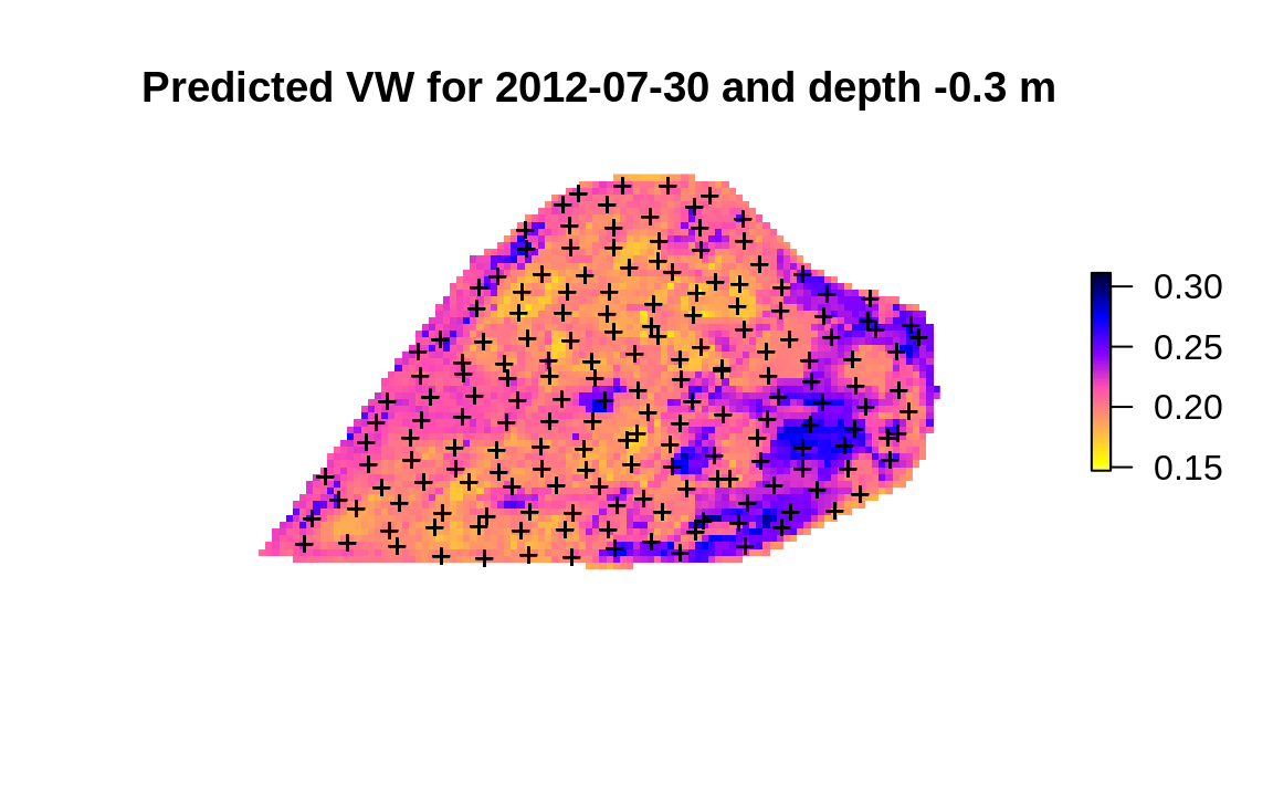

(#fig:map-eml.vw)Predicted soil water content based on spatiotemporal EML.

Because this is a spacetime dataset, we could also predict values of VW for longer periods (e.g. 100 days) then visualize changes using e.g. the animation package or similar.

In summary this study also demonstrate the importance of resampling point data using strict blocking of points that repeat in spacetime (measurement stations) is important to prevent from overfitting. The difference between models fitted using blocking per station and ignoring blocking can be drastic, hence how we define and use resampling is important (Meyer, Reudenbach, Hengl, Katurji, & Nauss, 2018).