1.1 Spatial data and spatial interpolation

Spatial and/or geospatial data is any data that is spatially referenced (in the case of geographical data referenced to Earth surface) i.e. \(X\) and \(Y\) coordinates are known. With the implementation of the GPS and Earth Observation technology, almost everything is becoming spatial data and hence tools such as Geographical Information Systems (GIS) and spatial analysis tools to process, analyze and visualize geospatial data are becoming essential.

Spatial interpolation and/or Spatial Prediction is a process of estimating values of the target variable over the whole area of interest by using some input training point data, algorithm and values of the covariates at new locations (Mitas & Mitasova, 1999). Interpolation results in images or maps, which can then be used for decision making or similar. There is a difference between interpolation and prediction: prediction can imply both interpolation and extrapolation. We will more commonly use the term spatial prediction in this tutorial, even though the term spatial interpolation has been more widely accepted (Mitas & Mitasova, 1999). In geostatistics, e.g. in the case of ordinary kriging, interpolation corresponds to cases where the location being estimated is surrounded by the sampling locations and is within the spatial auto-correlation range (Brown, 2015; Diggle & Ribeiro Jr, 2007). Prediction outside of the practical range (i.e. where prediction error exceeds the global variance) is referred to as spatial extrapolation. In other words, extrapolation is prediction at locations where we do not have enough statistical evidence (based on the statistical model) to make significant predictions.

1.2 Spatial interpolation using Ensemble Machine Learning

Ensemble Machine Learning (Ensemble ML) is an approach to modeling where, instead of using a single best learner, we use multiple strong learners and then combine their predictive capabilities into a single union. This can both lead to higher accuracy and robustness (Seni & Elder, 2010), but also helps with deriving model-free estimate of prediction errors through nonparametric techniques such as bootstrapping (C. Zhang & Ma, 2012). This way we can help decrease some methodological disadvantages of individual learners as shown in the previous example with synthetic data.

Ensemble ML can be used to fit models and generate predictions using points data the same way ordinary kriging is used to generate interpolations. Ensemble ML for predictive mapping in 2D and 3D is discussed in detail in the first chapter of the tutorial. Spatiotemporal interpolation using EML (2D+T, 3D+T) is at the order of magnitude more computational (Gasch et al., 2015) but it follows the same logic.

Ensemble ML based on stacking is implemented in the mlr package (Bischl et al., 2016) and can be initiated via the makeStackedLearner function e.g.:

m = mlr::makeStackedLearner(base.learners = lrns, 
              super.learner = "regr.ml", method = "stack.cv")

here the base learner predictions will be computed by 5-fold cross-validation (repeated re-fitting) and then used to determine the meta-learner. This algorithm is known as the “Super Learner” algorithm (Polley & van der Laan, 2010).

In the case of spatial prediction, we also want to block training points based on spatial proximity to prevent from producing bias predictions. For this we should know the range of spatial dependence for the model residuals or similar i.e.  something that can be derived by fitting a variogram, then limit the minimum spatial distance between training and validation points to avoid overfitting or similar (for more info refer to the Spatial Sampling tutorial).

To automate fitting of an Ensemble Machine Learning models for the purpose of spatial interpolation / prediction, one can now use the landmap package that combines:

• derivation of geographical distances,
  
• conversion of grids to principal components,
  
• automated filling of gaps in gridded data,
  
• automated fitting of variogram and determination of spatial auto-correlation structure,
  
• spatial overlay,
  
• model training using spatial Cross-Validation (Lovelace, Nowosad, & Muenchow, 2019),
  
• model stacking i.e. fitting of the final EML,

The concept of automating spatial interpolation until the level that almost no human interaction is required is referred to as “automated mapping” or automated spatial interpolation (Pebesma et al., 2011).

1.3 Spatiotemporal data

Spatiotemporal data is practically any data that is referenced in both space and time. This implies that the following coordinates are known:

• geographic location (longitude and latitude or projected \(X,Y\) coordinates);
  
• spatial location accuracy or size of the block / volume in the case of bulking of samples;
  
• height above the ground surface (elevation);
  
• start and end time of measurement (year, month, day, hour, minute etc.);

Consider for example daily temperature measured at some meteorological station. This would have the following coordinates:

temp = 22
lat = 44.56123
lon = 19.27734
delta.xy = 30
begin.time = "2013-09-02 00:00:00 CEST"
end.time = "2013-09-03 00:00:00 CEST"

which means that the measurement is fully spatiotemporally referenced with both \(X,Y\) location defined, delta.xy location accuracy known, and begin and end time of measurement specified (in this case temporal support is 1 day).

Analysis of spatiotemporal data is somewhat different from pure spatial analysis. Time is of course NOT just another spatial dimension i.e. it has specific properties and different statistical assumptions and methods apply to spatiotemporal data. For an introduction to spatiotemporal data in R please refer to the spacetime package tutorial (Pebesma, 2012).

Conceptually speaking, spatiotemporal datasets and corresponding databases can be matched with the two major groups of features (Erwig, Gu, Schneider, & Vazirgiannis, 1999): (1) moving or dynamic objects (discrete or vector geometries), and (2) dynamic regions (fields or continuous features). Distinct objects (entities) such as people, animals, vehicles and similar are best represented using vectors and trajectories (movement through time), and fields are commonly
represented using gridded structures. In the case of working with fields, we basically map either:

• dynamic changes in quantity or density of some material or chemical element,
  
• energy flux or any similar physical measurements,
  
• dynamic changes in probability of occurrence of some feature or object,

Spatiotemporal data can be best visualized 2D+T plots space-time cubes. One example of a spacetime cube is the following plot in Fig. 1.1 (T. Hengl, Heuvelink, Perčec-Tadić, & Pebesma, 2012; T. Hengl, Roudier, Beaudette, & Pebesma, 2015).

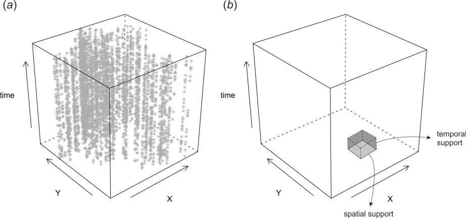
Figure 1.1: Space-time cube visualized in R: (a) cloud plot showing location of meteorological stations in Croatia, (b) illustration of spatial and temporal support in the space-time cube.

The plot above shows distribution of meteorological stations over Croatia, and then repeated measurements through time. This dataset is further used in the use-case examples to produce spatiotemporal predictions of daily temperatures.

1.4 Time-series analysis

Field of statistics dealing with modeling changes of variables through time, including predicting values beyond the training data (forecasting) is time-series analysis. Some systematic guides on how to run time-series analysis in R can be found here.

How a variable varies through time (time-series curves) can often be drastically different from how it changes in space (spatial patterns). In general, one can say that, for many environmental variables, variation of values through time can be separated into components such as:

• Long-term component (trend) determined by long-term geological and extraterrestrial processes,
• Seasonal monthly and/or daily component (seasonality) determined by Earth rotation and incoming sun radiation,
• Variation component which can be due to chaotic behavior and/or local factors (hence autocorrelated), and
• Pure noise i.e. measurement errors and similar,

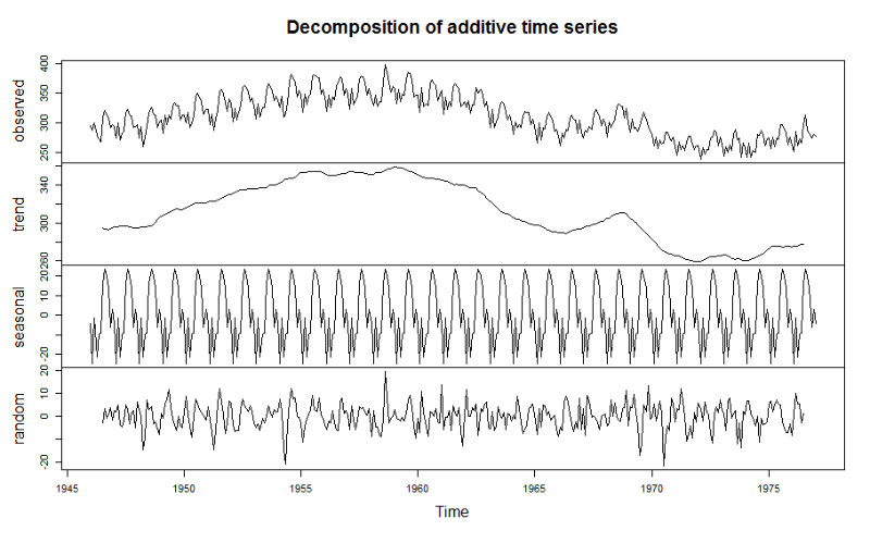
Figure 1.2: Illustration of decomposition of time-series into: (1) trend, (2) seasonality, and (3) random.

Consider for example the case of the land surface temperature. The long-term component is determined by variations in Earth’s orbit and/or Sun’s energy output resulting in gradual drops and rises of global mean temperature (glacials and interglacials). Fig. 1.3 shows example of a global temperature reconstruction from proxy data of Marcott, Shakun, Clark, & Mix (2013).

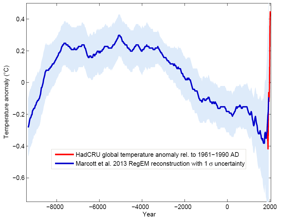
Figure 1.3: Global temperature reconstruction. This shows how global temperature varies on a long-term term scale. Graph by: Klaus Bitterman.

Seasonal i.e. monthly and daily components of variation of land surface temperature are also quite systematic. They are basically determined by Earth’s rotation and angles of Sun in relation to Earth’s surface. This is a relatively stable pattern that looks like sinusoidal curves or similar. The plot below shows variation of values of soil moisture and soil temperature at one meteo station in USA across multiple years (Gasch et al., 2015).

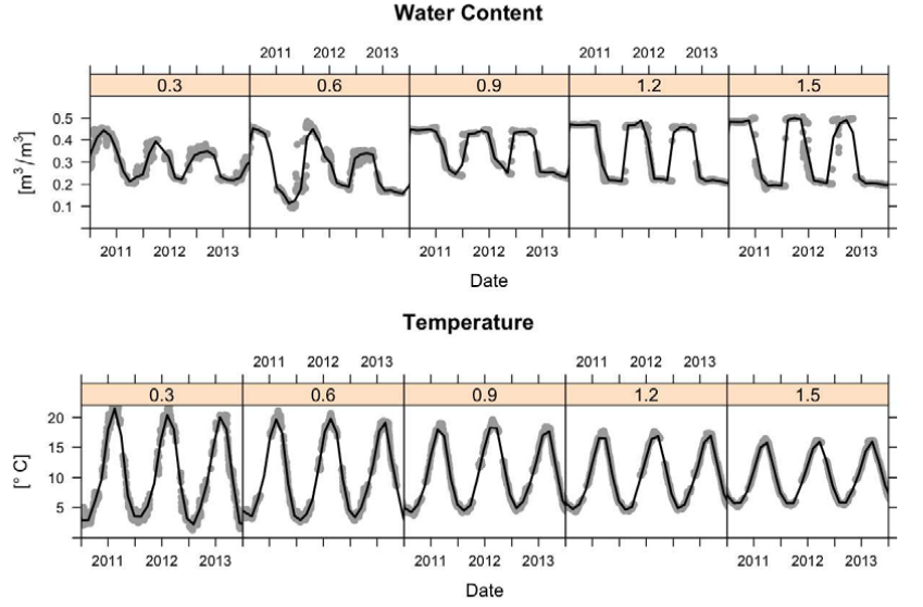
Figure 1.4: Sensor values from five depths (0.3, 0.6, 0.9, 1.2, and 1.5 m) at one station at Cook Agronomy Farm from January 2011–January 2014. The black line indicates locally fitted splines.

The data set in Fig. 1.4 is further discussed in the case studies to demonstrate 3D+T spatiotemporal modeling (Gasch et al., 2015). As we will see later, the seasonal daily and monthly part of variation is systematic and can be modeling using latitude, altitude and time/day of the year.

1.5 Visualizing spatiotemporal data

Spatial data is usually visualized using static or interactive maps (see e.g. mapview and/or tmap package). Spatiotemporal data (2D+T) is more complex to visualize than 2D data, while 3D+T data can even require special software (T. Hengl et al., 2015) before users can make any seamless interpretation.

There are three possible groups of ways to visualize spatiotemporal data:

1. Using static images showing trend parameters together with time-series plots at selected representative point locations.
   
2. Using time-slices or series of visualizations of the same spatial domain but changing in time (time-lapses).
   
3. Using animations or interactive plots with time-sliders allowing users to choose speed and direction of animation.

For an introduction to visualizing spatiotemporal and time-series data refer to Lamigueiro (2014). More complex visualization of spatiotemporal / dynamic geographic features is possible by using the https://geemap.org/ package (a Python package for interactive mapping with Google Earth Engine, ipyleaflet, and ipywidgets).

OpenLandMap.org also has multiple temporal datasets and users can interactive with the time-dimension by using time-slider implemented in OpenLayers and Geoserver (M. Kilibarda & Protić, 2019).

Figure 1.5: Visualization of land cover change using animation in www.OpenLandMap.org.

1.6 Spatiotemporal interpolation

Spatiotemporal interpolation and/or prediction implies that point samples are used to interpolate within the spacetime cube. This obviously assumes that enough point measurements are available, and which are spread in both space and time. We will show in this tutorial how Machine Learning can be used to interpolate values within the spacetime cube using real case-studies. Spatiotemporal interpolation using various kriging methods is implemented in the gstat package (Bivand, Pebesma, & Rubio, 2013), but is not addressed in this tutorial.

For success of spatiotemporal interpolation (in terms of prediction accuracy), the key is to recognize systematic component of variation in spacetime, which is usually possible if we can find relationship between the target variable and some EO data that is available as a time-series and covers the same spacetime cube of interest. Once we establish a significant relation between dynamic target and dynamic covariates, we can use the fitted model to predict anywhere in spacetime cube.

For more in-depth discussion on spatiotemporal data in R please refer to Wikle, Zammit-Mangion, & Cressie (2019). For in-depth discussion on spatial and spatiotemporal blocking for purpose of modeling building and cross-validation refer to Roberts et al. (2017).

1.7 Modeling seasonal components

Seasonality is the characteristic of the target variable to follow cyclical patterns such as in trigonometric functions. Such repeating patterns can happen at different time-scales:

• inter-annually,
  
• monthly or based on a season (spring, summer, autumn, winter),
  
• daily,
  
• hourly i.e. day-time and night-time patterns,

The monthly and daily seasonal component of variation is determined by Earth’s rotation and Sun’s angle. Milan Kilibarda et al. (2014) have shown that the seasonal component e.g. geometric Earth surface minimum and maximum daily temperature can be modeled, universally anywhere on globe, by using the following formula:

temp.from.geom <- function(fi, day, a=30.419375, 
                           b=-15.539232, elev=0, t.grad=0.6) {
  costeta = cos( (day-18 )*pi/182.5 + 2^(1-sign(fi) ) *pi) 
  cosfi = cos(fi*pi/180 )
  A = cosfi
  B = (1-costeta ) * abs(sin(fi*pi/180 ) )
  x = a*A + b*B - t.grad * elev / 100
  return(x)
}

where day is the day of year, fi is the latitude, the number 18 represents the coldest day in the northern and warmest day in the southern hemisphere, elev is the elevation in meter, 0.6 is the vertical temperature gradient per 100-m, and sign denotes the signum function that extracts the sign of a real number.

This formula accounts for different seasons at southern and northern hemisphere and can be basically applied on gridded surfaces to compute expected temperature at a given day. A simple example of min daily temperature is:

temp.from.geom(fi=52, day=120)
#> [1] 8.73603

If we plot this function for five consecutive years, we get something similar to the spline-fitted functions in the previous plot:

days = seq(1:(5*365))
plot(temp.from.geom(fi=52, day=days))

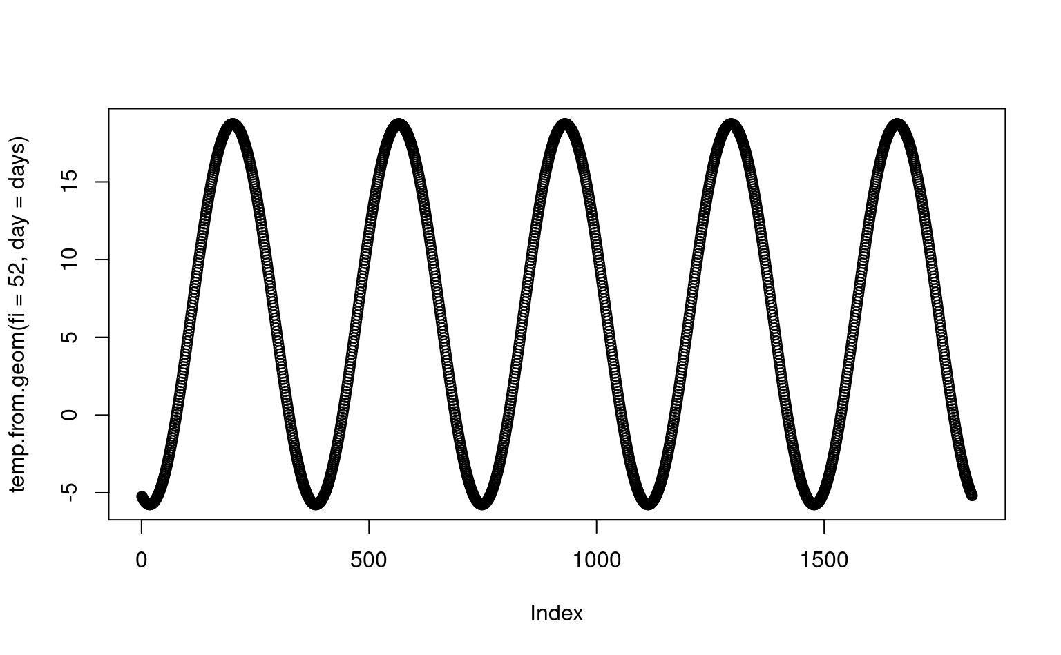
Figure 1.6: Geometric temperature function plot for a given latitude.

1.8 Predictive mapping using spatial and spatiotemporal ML in R

Standard spatiotemporal ML for predictive mapping typically includes the following steps (T. Hengl & MacMillan, 2019; T. Hengl et al., 2018):

1. Prepare training (points) data and data cube with all covariates ideally as an analysis-ready datacube.
2. Overlay points and create a regression-matrix.
   
3. Fine-tune initial model, reduce complexity and produce production-ready prediction model.
   
4. Run mapping accuracy assessment and determine prediction uncertainty including the per pixel uncertainty.
   
5. Generate predictions and save as maps.
6. Visualize predictions using web-GIS solutions.

Figure 1.7: General Machine Learning framework recommended for predictive mapping of vegetation / ecological / soil variables. Assuming full automation of modeling, 2nd-round samples can be used to gradually improve mapping accuracy.

1.9 Extrapolation and over-fitting problems of ML methods

Machine Learning has defacto become next-generation applied predictive modeling framework. ML techniques such as Random Forest (RF) have proven to over-perform vs more simple linear statistical methods, especially where the datasets are large, complex and target variable follows complex relationship with covariates (T. Hengl et al., 2018). Random Forest comes at a cost however. There are four main practical disadvantages of RF:

• Depending on data and assumptions about data, it can over-fit values without an analyst even noticing it.
  
• It predicts well only within the feature space with enough training data. Extrapolation i.e. prediction outside the training space can lead to poor performance (Meyer & Pebesma, 2021).
  
• It can be computationally expensive with computational load increasing exponentially with the number of covariates.
  
• It requires quality training data and is highly sensitive to blunders and typos in the data.

Read more about extrapolation problems of Random Forest in this post.

In the following section we will demonstrate that indeed RF can overfit data and can have serious problems with predicting in the extrapolation space. Consider for example the following small synthetic dataset assuming simple linear relationship (see original post by Dylan Beaudette):

set.seed(200)
n = 100
x <- 1:n
y <- x + rnorm(n = 50, mean = 15, sd = 15)

If we fit a simple Ordinary Least Square model to this data we get:

m0 <- lm(y ~ x)
summary(m0)
#> 
#> Call:
#> lm(formula = y ~ x)
#> 
#> Residuals:
#>      Min       1Q   Median       3Q      Max 
#> -27.6093  -6.4396   0.6437   6.7742  26.7192 
#> 
#> Coefficients:
#>             Estimate Std. Error t value Pr(>|t|)    
#> (Intercept) 14.84655    2.37953   6.239 1.12e-08 ***
#> x            0.97910    0.04091  23.934  < 2e-16 ***
#> ---
#> Signif. codes:  0 '***' 0.001 '**' 0.01 '*' 0.05 '.' 0.1 ' ' 1
#> 
#> Residual standard error: 11.81 on 98 degrees of freedom
#> Multiple R-squared:  0.8539, Adjusted R-squared:  0.8524 
#> F-statistic: 572.9 on 1 and 98 DF,  p-value: < 2.2e-16

we see that the model explains about 85% of variation in the data and that the RMSE estimated by the model (residual standard error) matches very well the noise component we have inserted on purpose using the rnorm function.

If we fit a Random Forest model to this data we get:

library(randomForest)
#> randomForest 4.6-14
#> Type rfNews() to see new features/changes/bug fixes.
#> 
#> Attaching package: 'randomForest'
#> The following object is masked from 'package:ranger':
#> 
#>     importance
rf = randomForest::randomForest(data.frame(x=x), y, nodesize = 5, keep.inbag = TRUE)
rf
#> 
#> Call:
#>  randomForest(x = data.frame(x = x), y = y, nodesize = 5, keep.inbag = TRUE) 
#>                Type of random forest: regression
#>                      Number of trees: 500
#> No. of variables tried at each split: 1
#> 
#>           Mean of squared residuals: 202.6445
#>                     % Var explained: 78.34

Next, we can estimate the prediction errors using the method of Lu & Hardin (2021), which is available via the forestError package:

library(forestError)
rmse <- function(a, b) {  sqrt(mean((a - b)^2)) }
dat <- data.frame(x,y)
newdata <- data.frame(
  x = -100:200
)
newdata$y.lm <- predict(m0, newdata = newdata)
## prediction error from forestError:
quantiles = c((1-.682)/2, 1-(1-.682)/2)
pr.rf = forestError::quantForestError(rf, X.train=data.frame(x=x), 
                                      X.test=data.frame(x = -100:200), 
                                      Y.train=y, alpha = (1-(quantiles[2]-quantiles[1])))
newdata$y.rf <- predict(rf, newdata = newdata)
rmse.lm <- round(rmse(y, predict(m0)), 1)
rmse.rf <- round(rmse(y, predict(rf)), 1)
rmse.lm; rmse.rf
#> [1] 11.7
#> [1] 14.2

This shows that RF estimates higher RMSE than linear model. However, if we visualize the two models against each other we see that indeed RF algorithm seems to over-fit this specific data:

leg.txt <- sprintf("%s (%s)", c('lm', 'RF'), c(rmse.lm, rmse.rf))
par(mar = c(0, 0, 0, 0), fg = 'black', bg = 'white')
plot(y ~ x, xlim = c(-25, 125), ylim = c(-50, 150), type = 'n', axes = FALSE)
grid()
points(y ~ x, cex = 1, pch = 16, las = 1)
lines(y.lm ~ x, data = newdata, col = 2, lwd = 2)
lines(y.rf ~ x, data = newdata, col = 4, lwd = 2)
lines(newdata$x, pr.rf$estimates$lower_0.318, lty=2,col=4)
lines(newdata$x, pr.rf$estimates$upper_0.318, lty=2,col=4)
legend('bottom', legend = leg.txt, lwd = 2, lty = 1, col = c(2, 4, 3), horiz = TRUE, title = 'RMSE')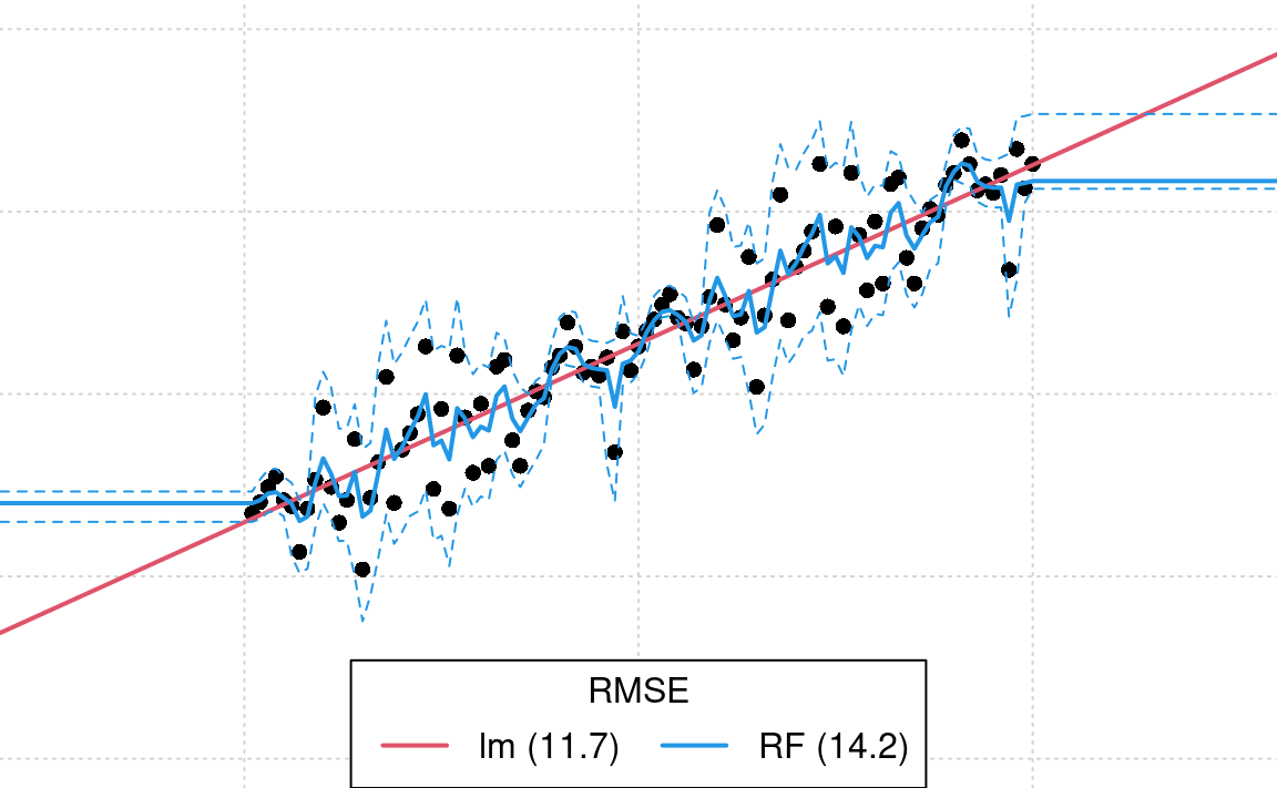

Figure 1.8: Difference in model fits for sythetic data: lm vs RF. In this case we know that RF (blue line) is overfitting and under-estimating the prediction error in the extrapolation space. Dotted line shows respective 1 std. prediction interval for RF.

RF basically tries to fit relationship even to the pure noise component of variation (we know it is pure noise because we have generated it using the rnorm function). This is obvious over-fitting as we do not want to model something which is purely random.

Extrapolation would not maybe be so much of a problem in the example above if the prediction intervals from the forestError package expressed more realistically that the predictions deviate from the linear structure in the data. Assuming that, after the prediction, one would eventually collect ground-truth data for the RF model above, these would probably show that the prediction error / prediction intervals are completely off. Most traditional statisticians would consider these too-narrow and over-optimistic and the fitted line over-fit, and hence any further down the pipeline over-optimistic prediction uncertainty can result in decision makers being over-confident, leading to wrong decisions, and consequently making users losing any confidence in RF. For an in-depth discussion on extrapolation problems and Area of Applicability of Machine Learning models please refer to Meyer & Pebesma (2021).

A possible solution to the problem above is to, instead of using only one learners, we use multiple learners and then apply robust cross-validation that prevents the target model from over-fitting. This can be implemented efficiently, for example, by using the mlr package (Bischl et al., 2016). We can run an Ensemble Model by applying the following four steps. First, we define the task of interest and a combination of learners i.e. so-called base learners:

library(mlr)
library(kernlab)
#> 
#> Attaching package: 'kernlab'
#> The following objects are masked from 'package:raster':
#> 
#>     buffer, rotated
library(mboost)
#> Loading required package: parallel
#> Loading required package: stabs
#> 
#> Attaching package: 'stabs'
#> The following object is masked from 'package:mlr':
#> 
#>     subsample
#> This is mboost 2.9-2. See 'package?mboost' and 'news(package  = "mboost")'
#> for a complete list of changes.
#> 
#> Attaching package: 'mboost'
#> The following object is masked from 'package:glmnet':
#> 
#>     Cindex
#> The following objects are masked from 'package:raster':
#> 
#>     cv, extract
library(landmap)
SL.library = c("regr.ranger", "regr.glm", "regr.gamboost", "regr.ksvm")
lrns <- lapply(SL.library, mlr::makeLearner)
tsk <- mlr::makeRegrTask(data = dat, target = "y")

In this case we use basically four very different models: RF (ranger), linear model (glm), Gradient boosting (gamboost) and Support Vector Machine (kvsm). Second, we train the Ensemble model by using the stacking approach:

init.m <- mlr::makeStackedLearner(lrns, method = "stack.cv", super.learner = "regr.lm", resampling=mlr::makeResampleDesc(method = "CV"))
eml = train(init.m, tsk)
summary(eml$learner.model$super.model$learner.model)
#> 
#> Call:
#> stats::lm(formula = f, data = d)
#> 
#> Residuals:
#>      Min       1Q   Median       3Q      Max 
#> -28.0474  -7.0473  -0.4075   7.2528  28.6083 
#> 
#> Coefficients:
#>               Estimate Std. Error t value Pr(>|t|)    
#> (Intercept)   -0.86179    3.01456  -0.286  0.77560    
#> regr.ranger   -0.27294    0.24292  -1.124  0.26402    
#> regr.glm       4.75714    1.09051   4.362 3.27e-05 ***
#> regr.gamboost -3.55134    1.14764  -3.094  0.00259 ** 
#> regr.ksvm      0.08578    0.28482   0.301  0.76394    
#> ---
#> Signif. codes:  0 '***' 0.001 '**' 0.01 '*' 0.05 '.' 0.1 ' ' 1
#> 
#> Residual standard error: 11.25 on 95 degrees of freedom
#> Multiple R-squared:  0.8714, Adjusted R-squared:  0.8659 
#> F-statistic: 160.9 on 4 and 95 DF,  p-value: < 2.2e-16

The results show that ranger and ksvm basically under-perform and are in fact not significant for this specific data i.e. could be probably omitted from modeling.

Note that, for stacking of multiple learners we use a separate model (a meta-learner) which is in this case a simple linear model. We use a simple model because we assume that the non-linear relationships have already been modeled via complex models such as ranger, gamboost and/or ksvm.

Next, we need to estimate mapping accuracy and prediction errors for Ensemble predictions. This is not trivial as there are no simple derived formulas. We need to use a non-parametric approach basically and this can be very computational. A computationally interesting approach is to first estimate the (global) mapping accuracy, then adjust the prediction variance from multiple base learners:

newdata$y.eml = predict(eml, newdata = newdata)$data$response
m.train = eml$learner.model$super.model$learner.model$model
m.terms = eml$learner.model$super.model$learner.model$terms
eml.MSE0 = matrixStats::rowSds(as.matrix(m.train[,all.vars(m.terms)[-1]]), na.rm=TRUE)^2
eml.MSE = deviance(eml$learner.model$super.model$learner.model)/df.residual(eml$learner.model$super.model$learner.model)
## correction factor / mass-preservation of MSE
eml.cf = eml.MSE/mean(eml.MSE0, na.rm = TRUE)
eml.cf
#> [1] 9.328646

This shows that variance of the learners is about 10 times smaller than the actual CV variance. Again, this proves that many learners try to fit data very closely so that variance of different base learners is often smoothed out.

Next, we can predict values and prediction errors at all new locations:

pred = mlr::getStackedBaseLearnerPredictions(eml, newdata=data.frame(x = -100:200))
rf.sd = sqrt(matrixStats::rowSds(as.matrix(as.data.frame(pred)), na.rm=TRUE)^2 * eml.cf)
rmse.eml <- round(sqrt(eml.MSE), 1)

and the plot the results of fitting linear model vs EML:

leg.txt <- sprintf("%s (%s)", c('lm', 'EML'), c(rmse.lm, rmse.eml))
par(mar = c(0, 0, 0, 0), fg = 'black', bg = 'white')
plot(y ~ x, xlim = c(-25, 125), ylim = c(-50, 150), type = 'n', axes = FALSE)
grid()
points(y ~ x, cex = 1, pch = 16, las = 1)
lines(y.lm ~ x, data = newdata, col = 2, lwd = 2)
lines(y.eml ~ x, data = newdata, col = 4, lwd = 2)
lines(newdata$x, newdata$y.eml+rmse.eml+rf.sd, lty=2, col=4)
lines(newdata$x, newdata$y.eml-(rmse.eml+rf.sd), lty=2, col=4)
legend('bottom', legend = leg.txt, lwd = 2, lty = 1, col = c(2, 4, 3), horiz = TRUE, title = 'RMSE')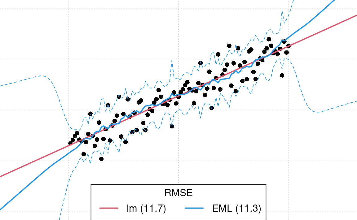

Figure 1.9: Difference in model fits for sythetic data: lm vs Ensemble ML.

From the plot above, we see that the prediction error intervals in the extrapolation space are now wider (compare with Fig. 1.8), and this reflects much better what we would expect than if we have only used the forestError package.

In summary: it appears that combining linear and non-linear tree-based models in an Ensemble ML framework helps both: decrease over-fitting and produce more realistic predictions of uncertainty / prediction intervals. The Ensemble ML framework correctly identifies linear models as being more important than random forest or similar. Hopefully, this provides enough evidence to convince you that Ensemble ML is potentially interesting for use as a generic solution for spatial and spatiotemporal interpolation and extrapolation.