5 Spatiotemporal Machine Learning for Species Distribution Modeling

You are reading the work-in-progress Spatial and spatiotemporal interpolation using Ensemble Machine Learning. This chapter is currently draft version, a peer-review publication is pending. You can find the polished first edition at https://opengeohub.github.io/spatial-prediction-eml/.

5.1 Species Distribution Modeling

Species Distribution Modeling (SDM) and/or Mapping aims at explaining and mapping distribution of species as a function of ecological, environmental conditions and/or human influence. Typical steps in SDM include (Hijmans, 2019):

Prepare locations of occurrence of a species or species density;
Prepare environmental predictor variables (climate, terrain, surface water);
Fit a SDM model that can be used either to predict natural habitat / Niche and/or occurrence probability;
Predict habitat / occurrence probability across the region of interest (and perhaps for a future or past climate).

Modeling species distribution is different from mapping quantitative soil properties and/or land surface temperature described in previous chapters. Species training data often comes with specific properties that include (Fois, Cuena-Lombraña, Fenu, & Bacchetta, 2018; Martinez-Minaya, Cameletti, Conesa, & Pennino, 2018):

Dealing with occurrence-only records: biologists / ecologists often only record where some species was observed;
Species and their dynamics is often complex: some species such as migratory birds change location seasonaly;
Modeling distribution of species such as birds or similar animals and insects in spacetime context is highly complex as various levels of chaotic behavior apply;

In recent years there has been an increasing interest in using Machine Learning for species distribution modeling, especially to model disease outbreaks. A review of ML methods for SDM is available also in J. Zhang & Li (2017). In this chapter we describe a scalable framework for predicting species occurrences based on the Ensemble Machine Learning described in the previous chapter. The target variables of interest in the case of SDM are usually (a) probability of occurrence and/or (b) species density (number of individuals per area) and/or (c) habitat suitability indices. As covariates for SDM we use time-series of Earth Observation images and similar climatic and terrain-based images.

Extending spatiotemporal Ensemble ML to modeling species distribution is not trivial. In order to be able to interpolate species distribution, probability of occurrence and/or density of species in space-time using Ensemble ML, we can not simply import and model occurrence-only data as these miss any quantities or states. We need to provide instead run several steps to make data suited for ML. For example, if absence training points are not available, we can use various method do derive most likely locations where certain species do NOT occur i.e. are highly unlikely to occur due to ecological limitations such as minimum winter temperature minimum rainfall or similar. These are referred to as the pseudo-absence training points. Hence, we will first show how to generate pseudo-absence data using the maxlike package, then after enough of occurrence and absence records are available, we apply standard ML steps.

5.2 Tiger Mosquito over Europe

The tiger mosquito (Aedes albopictus) is a vector species for many different viruses including those responsible for dengue fever, Zika and chikungunya. The natural habitat of this species was limited in the past, however, in the recent time, this species has spread to many countries through the transport of goods and international travel e.g. shipping routes or similar (Benedict, Levine, Hawley, & Lounibos, 2007; Da Re, Montecino-Latorre, Vanwambeke, & Marcantonio, 2021). The R package dynamAedes contains stochastic, time-discrete and spatially-explicit population dynamical models for Aedes sp. invasive species (Da Re, Van Bortel, et al., 2021).

We can obtain occurrences of the Aedes albopictus by either using the rgbif::occ_data function, or by downloading the CSV file from the GBIF website. A local copy of the occurrences for Europe can be loaded by using:

## occ = rgbif::occ_data(taxonKey=1651430, hasCoordinate = TRUE, year = '2000,2022')
occ = readRDS("./input/gbif_aedes_albopictus_mood.rds")
str(occ)
#> 'data.frame':    13834 obs. of  9 variables:
#>  $ occurrenceID                 : chr  "https://observation.org/observation/226030224" "https://observation.org/observation/229897504" "https://observation.org/observation/222737616" "https://observation.org/observation/221356176" ...
#>  $ scientificName               : chr  "Aedes albopictus (Skuse, 1894)" "Aedes albopictus (Skuse, 1894)" "Aedes albopictus (Skuse, 1894)" "Aedes albopictus (Skuse, 1894)" ...
#>  $ individualCount              : num  1 1 1 1 10 125 22 3 2 2 ...
#>  $ Date                         : Date, format: "2021-09-21" "2021-07-22" ...
#>  $ coordinateUncertaintyInMeters: num  43 25 356 4 NA NA NA NA NA NA ...
#>  $ decimalLongitude             : num  3.206 -0.349 4.863 -0.647 12.726 ...
#>  $ decimalLatitude              : num  42 43.3 45.8 38.1 42.1 ...
#>  $ Year                         : int  2021 2021 2021 2021 2020 2020 2020 2020 2020 2020 ...
#>  $ olc_c                        : chr  "8FH5X6G4+VF3" "8CMX8M42+Q8G" "8FQ6QVW7+M8J" "8CCX49J3+95Q" ...

To visualize the mosquito point data over Europe we can use e.g.:

library(spacetime)
library(plotKML)
sp_ST <- STIDF(SpatialPoints(occ[,c("decimalLongitude", "decimalLatitude")], proj4string = CRS("EPSG:4326")), 
               occ$Date, data.frame(individualCount=occ$individualCount))
data(SAGA_pal)
## plot in Google Earth:
plotKML(sp_ST, colour_scale=SAGA_pal[[1]])

Figure 5.1: Spatiotemporal visualization of the GBIF occurrence records of the Tiger mosquito.

This shows that mosquito seems to be concentrated in the southern Europe, primarily along coast-line, although some adults have been spotted also in the Northern Europe. Note also that the mosquito seems to be continuously spreading across Europe, however, we are not sure if this is also just because there are more records in GBIF coming from the last 5 years.

5.3 Generating pseudo-absence data

Pseudo-absence points can be generated in several ways, but most commonly by using occurrence-only models, expert knowledge and/or geosurveys (Iturbide et al., 2015; Lobo, Jiménez-Valverde, & Hortal, 2010).
To generate pseudo-absence data we can use the maxlike package. First, we need to prepare enough ecological information that can help us map habitat of the species using all records for Europe. In the local folder we can find:

eco.tifs = list.files("./input/mood4km/static", glob2rx("*.tif$"), full.names=TRUE)
basename(eco.tifs)
#>  [1] "clm_bioclim.1_chelsa.climate_m_4km_s0..0cm_1980..2010_mood_v2.1.tif"      
#>  [2] "clm_bioclim.12_chelsa.climate_m_4km_s0..0cm_1980..2010_mood_v2.1.tif"     
#>  [3] "clm_bioclim.13_chelsa.climate_m_4km_s0..0cm_1980..2010_mood_v2.1.tif"     
#>  [4] "clm_bioclim.14_chelsa.climate_m_4km_s0..0cm_1980..2010_mood_v2.1.tif"     
#>  [5] "clm_bioclim.5_chelsa.climate_m_4km_s0..0cm_1980..2010_mood_v2.1.tif"      
#>  [6] "clm_bioclim.6_chelsa.climate_m_4km_s0..0cm_1980..2010_mood_v2.1.tif"      
#>  [7] "clm_lst_mod11a2.nighttime.m01_p50_4km_s0..0cm_2000..2021_mood_v1.2.tif"   
#>  [8] "clm_lst_mod11a2.nighttime.m03_p50_4km_s0..0cm_2000..2021_mood_v1.2.tif"   
#>  [9] "clm_lst_mod11a2.nighttime.m06_p50_4km_s0..0cm_2000..2021_mood_v1.2.tif"   
#> [10] "clm_lst_mod11a2.nighttime.m09_p50_4km_s0..0cm_2000..2021_mood_v1.2.tif"   
#> [11] "clm_snow.prob_esacci.dec_p.90_4km_s0..0cm_2000..2012_mood_v2.0.tif"       
#> [12] "clm_snow.prob_esacci.feb_p.90_4km_s0..0cm_2000..2012_mood_v2.0.tif"       
#> [13] "clm_snow.prob_esacci.jan_p.90_4km_s0..0cm_2000..2012_mood_v2.0.tif"       
#> [14] "dtm_elevation_glo90.copernicus_m_4km_s0..0cm_2019_epsg.4326_mood_v1.0.tif"

i.e. CHELSA Climate Bioclim layers mean annual air temperature, annual precipitation amount and similar, MODIS Long-term nighttime Land Surface Temperatures for months 1, 3, 6 and 9, snow probability images for winter months and DTM elevation model from Copernicus. We can load the stack of rasters into R and use principal components to reduce overlap between different layers:

#gc()
g4km = raster::stack(eco.tifs)
g4km = as(g4km, "SpatialGridDataFrame")
cc.4km = complete.cases(g4km@data)
g4km = as(g4km, "SpatialPixelsDataFrame")
g4km = g4km[cc.4km,]
#summary(cc.4km)
## 2.2M pixels
#plot(g4km[14])
g4km.spc = landmap::spc(g4km)
#> Converting covariates to principal components...

Next, we can fit a maxlike model for occurrence probability using presence only data, and predict values at all locations:

occ.sp = occ[,c("decimalLongitude","decimalLatitude","Year","olc_c")]
occ.sp = occ.sp[!duplicated(occ.sp$olc_c),]
coordinates(occ.sp) <- c("decimalLongitude", "decimalLatitude")
proj4string(occ.sp) <- CRS("+init=epsg:4326")
occ.sp <- spTransform(occ.sp, "EPSG:3035")

#gc()
max.fm <- stats::as.formula(paste("~", paste(names(g4km.spc@predicted[1:12]), collapse="+")))
max.ml <- maxlike::maxlike(formula=max.fm, rasters=raster::stack(g4km.spc@predicted[1:12]), points=occ.sp@coords, method="BFGS", savedata=TRUE)
#ment.ml <- dismo::maxent(raster::stack(g4km.spc@predicted[1:12]), occ.sp@coords)
## bug in "maxlike" (https://github.com/rbchan/maxlike/issues/1); need to replace this 'by hand':
max.ml$call$formula <- max.fm
## TH: this operation can be time consuming and is not recommended for large grids
max.ml.p <- predict(max.ml)
max.ml.p <- methods::as(max.ml.p, "SpatialGridDataFrame")
plot(max.ml.p)

The resulting maps produced using maxlike are shown below.

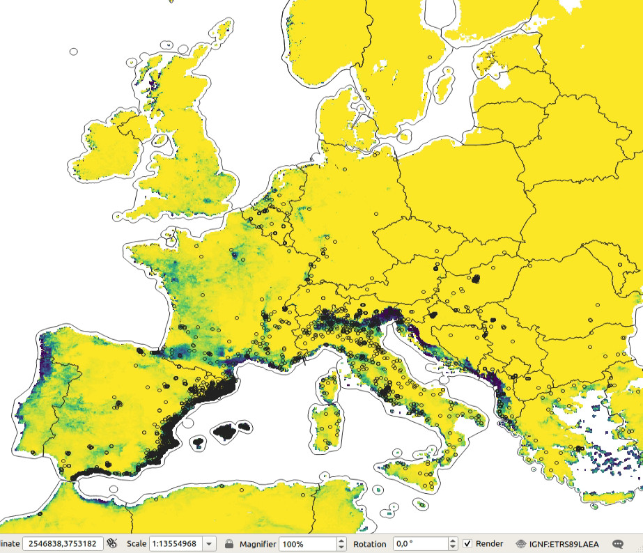
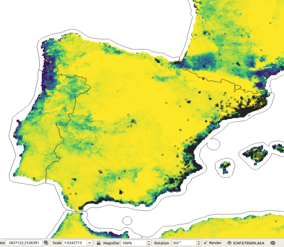
Predicted probability of occurence for Tiger mosquito based on the maxent analysis. Darker-green areas indicated close to 100% probability of occurrence.

Figure 5.2: Predicted probability of occurence for Tiger mosquito based on the maxent analysis. Darker-green areas indicated close to 100% probability of occurrence.

The maxlike occurrence probability map indicates that the Tiger mosquito seems to prefer coastal areas and is probably limited by the winter temperatures. The minimum temperature for survival of the mosquito adults is about 3–4 C degrees, for mosquito eggs minimum temperature is lower but still should be above -4 degrees (Da Re, Montecino-Latorre, et al., 2021). Note for habitat suitability analysis one could also use the maxent algorithm or do analysis in both maxlike and maxent and then produce an ensemble estimate.

Next, we can generate a reasonable number of pseudo-absences (as a rule of thumb, number of the generated pseudo-absences should not exceed 10% to 20% of the actual number of occurrence points):

max.ml.p = rgdal::readGDAL("./output/occ.prob_aedes_albopictus.tif")
## insert 0 values for all occurrences before the date:
max.ml.p$absence = ifelse(max.ml.p$band1==100, 1, NA)
dens.var <- spatstat.geom::as.im(sp::as.image.SpatialGridDataFrame(max.ml.p["absence"]))
pnts.new <- rpoint(600, f=dens.var)

A single realization of 600 simulated pseudo-absences is shown below:

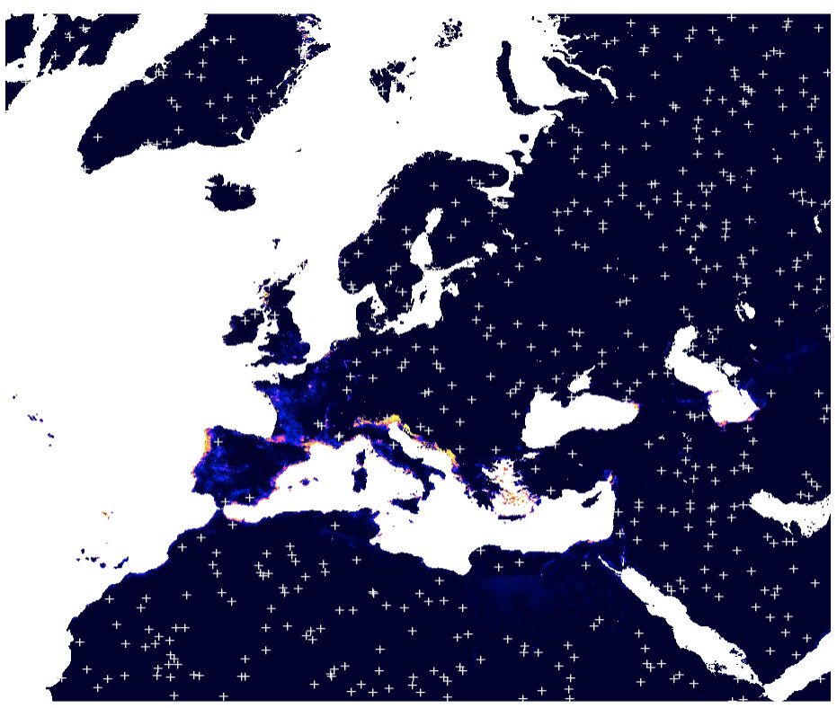
Figure 5.3: Simulated pseudo-absences based on the maxent analysis (predictions in the background).

Note we only use pixels that have 0 probability of occurrence based on the maxlike results. This way we prevent from introducing any bias into further modeling. Once we have generated pseudo-absences, we can bind all 1 and 0 records together to produce a regression and/or classification matrix, and which can then be used to fit ML models.

In the case of the GBIF data two possible target variables could be used:

Individual counts i.e. number of adults observed at location;
Occurrence / absence states i.e. 0/1 values;

We focus further on modeling the 0/1 states and predicting probabilities. This puts this ML exercises into the category of ML for classification.

5.4 Modeling occurrence-only records using Random Forest

Thanks to the package solitude it is possible to predict probability of distribution of species by using the occurrence-only data. The method is explained in detail in Liu, Ting, & Zhou (2012) and Hariri, Kind, & Brunner (2019). Solitude builds on top of the ranger package hence it is suitable also for larger datasets. To fit the model we do not need to specify any target column but we ONLY specify a matrix of covariates at occurrence locations:

library(solitude)
occ.ov = sp::over(occ.sp, g4km.spc@predicted[1:12])
occ.ov = occ.ov[complete.cases(occ.ov),]
#head(occ.ov)
iso = isolationForest$new()
iso$fit(dataset = occ.ov)
#> INFO  [18:54:39.156] dataset has duplicated rows 
#> INFO  [18:54:39.202] Building Isolation Forest ...  
#> INFO  [18:54:39.293] done 
#> INFO  [18:54:39.296] Computing depth of terminal nodes ...  
#> INFO  [18:54:39.898] done 
#> INFO  [18:54:40.146] Completed growing isolation forest

The fitted model shows:

iso$forest
#> Ranger result
#> 
#> Call:
#>  ranger::ranger(x = dataset, y = yy, mtry = ncol(dataset) - 1L,      min.node.size = 1L, splitrule = "extratrees", num.random.splits = 1L,      num.trees = self$num_trees, replace = self$replace, sample.fraction = private$sample_fraction,      respect.unordered.factors = self$respect_unordered_factors,      num.threads = self$nproc, seed = self$seed, max.depth = self$max_depth) 
#> 
#> Type:                             Regression 
#> Number of trees:                  100 
#> Sample size:                      9253 
#> Number of independent variables:  12 
#> Mtry:                             11 
#> Target node size:                 1 
#> Variable importance mode:         none 
#> Splitrule:                        extratrees 
#> Number of random splits:          1 
#> OOB prediction error (MSE):       7183789 
#> R squared (OOB):                  -0.006752571

These numbers are somewhat difficult to interpret with R-square being close to 0. We can produce predictions of the anomaly scores (the likelihood that a point is an outlier) for every location based on the fitted model using:

pred.iso = iso$predict(data=g4km.spc@predicted@data[,1:12])
g4km$anomaly_score = pred.iso$anomaly_score*100
rgdal::writeGDAL(g4km["anomaly_score"], "./output/aedes_anomaly_score_4km.tif", type="Int16", 
          mvFlag=-32768, options=c("COMPRESS=DEFLATE"))

this gives the following output:

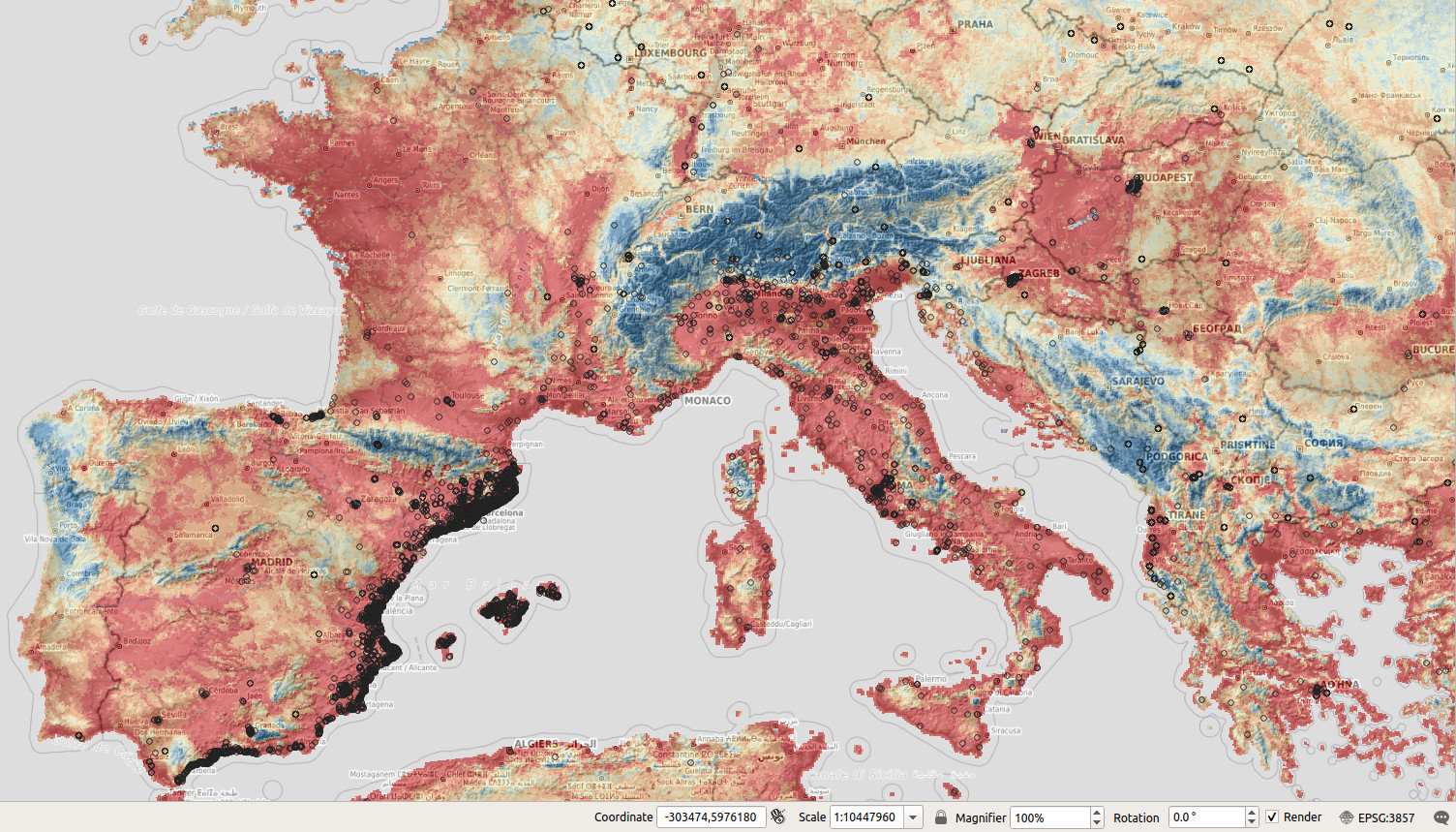
Figure 5.4: Predicted anomaly score based on the solitude package for the Tiger mosquito. Red values indicate low anomaly.

In general there seems to be a large difference in the outputs (spatial patterns) of maxlike and solitude, nevertheless the predictions seem to show overall similar patterns: both maxlike and solitude predict that the temperature regime seem to be the most limiting factor for the Tiger mosquito. Note, however, that solitude by default only returns anomaly scores, which are abstract and should not be interpreted as probability of occurrence at all.

5.5 Modeling distribution of mosquitos through time

Next we can overlay training points (occurrences / adult counts and pseudo-absences) in spacetime to produce a spatiotemporal regression-matrix. The total list of layers for Europe (MOOD Horizon 2020 project) available as Cloud-Optimized GeoTIFFs is documented in:

cov.lst = read.csv("./input/mood_layers1km.csv")
str(cov.lst)
#> 'data.frame':    454 obs. of  5 variables:
#>  $ n          : int  1 2 3 4 5 6 7 8 9 10 ...
#>  $ filename   : chr  "https://s3.eu-central-1.wasabisys.com/mood/CRP/lcv_globalcropland_bowen.et.al_p_1km_s0..0cm_2000_mood_v0.1.tif" "https://s3.eu-central-1.wasabisys.com/mood/CRP/lcv_globalcropland_bowen.et.al_p_1km_s0..0cm_2001_mood_v0.1.tif" "https://s3.eu-central-1.wasabisys.com/mood/CRP/lcv_globalcropland_bowen.et.al_p_1km_s0..0cm_2002_mood_v0.1.tif" "https://s3.eu-central-1.wasabisys.com/mood/CRP/lcv_globalcropland_bowen.et.al_p_1km_s0..0cm_2003_mood_v0.1.tif" ...
#>  $ size       : chr  "9.7 Mb" "9.7 Mb" "9.7 Mb" "9.8 Mb" ...
#>  $ source_doi : chr  "http://doi.org/10.5194/essd-13-5403-2021" "http://doi.org/10.5194/essd-13-5403-2021" "http://doi.org/10.5194/essd-13-5403-2021" "http://doi.org/10.5194/essd-13-5403-2021" ...
#>  $ description: chr  "Cropland fraction historic" "Cropland fraction historic" "Cropland fraction historic" "Cropland fraction historic" ...

To connect to the layers and extract values at point locations we can use:

library(terra)
tif = paste0("/vsicurl/", cov.lst$filename[2])
r = rast(tif)
#> Warning in new_CppObject_xp(fields$.module, fields$.pointer, ...): GDAL Message
#> 1: HTTP response code on
#> https://s3.eu-central-1.wasabisys.com/mood/CRP/lcv_globalcropland_bowen.et.al_p_1km_s0..0cm_2001_mood_v0.1.tif.aux.xml:
#> 403
#> Warning in new_CppObject_xp(fields$.module, fields$.pointer, ...): GDAL Message
#> 1: HTTP response code on
#> https://s3.eu-central-1.wasabisys.com/mood/CRP/lcv_globalcropland_bowen.et.al_p_1km_s0..0cm_2001_mood_v0.1.aux:
#> 403
#> Warning in new_CppObject_xp(fields$.module, fields$.pointer, ...): GDAL Message
#> 1: HTTP response code on
#> https://s3.eu-central-1.wasabisys.com/mood/CRP/lcv_globalcropland_bowen.et.al_p_1km_s0..0cm_2001_mood_v0.1.AUX:
#> 403
#> Warning in new_CppObject_xp(fields$.module, fields$.pointer, ...): GDAL Message
#> 1: HTTP response code on
#> https://s3.eu-central-1.wasabisys.com/mood/CRP/lcv_globalcropland_bowen.et.al_p_1km_s0..0cm_2001_mood_v0.1.tif.aux:
#> 403
#> Warning in new_CppObject_xp(fields$.module, fields$.pointer, ...): GDAL Message
#> 1: HTTP response code on
#> https://s3.eu-central-1.wasabisys.com/mood/CRP/lcv_globalcropland_bowen.et.al_p_1km_s0..0cm_2001_mood_v0.1.tif.AUX:
#> 403
r
#> class       : SpatRaster 
#> dimensions  : 7360, 7845, 1  (nrow, ncol, nlyr)
#> resolution  : 1000, 1000  (x, y)
#> extent      : 867000, 8712000, -484000, 6876000  (xmin, xmax, ymin, ymax)
#> coord. ref. : +proj=laea +lat_0=52 +lon_0=10 +x_0=4321000 +y_0=3210000 +ellps=GRS80 +units=m +no_defs 
#> source      : lcv_globalcropland_bowen.et.al_p_1km_s0..0cm_2001_mood_v0.1.tif 
#> name        : lcv_globalcropland_bowen.et.al_p_1km_s0..0cm_2001_mood_v0.1

To get values of pixels at some location we can fetch values without downloading the complete rasters e.g.:

terra::extract(r, data.frame(x=3828332, y=2315068))
#>   ID lcv_globalcropland_bowen.et.al_p_1km_s0..0cm_2001_mood_v0.1
#> 1  1                                                          24

Opening Cloud-Optimized GeoTIFF layers in QGIS. The total size of layers exceeds 30GB so it is more efficient to access data using the COG-architecture and S3 services.

Figure 5.5: Opening Cloud-Optimized GeoTIFF layers in QGIS. The total size of layers exceeds 30GB so it is more efficient to access data using the COG-architecture and S3 services.

The spacetime overlay process can be computational hence we have already pre-computed the regression / classification matrix:

source("mood_functions.R")
rm.all = readRDS("./input/regmatrix_aedes_1km.rds")
dim(rm.all)
#> [1] 18234   183

This is now a relatively large matrix with basically diversity of Earth Observation and climatic time-series of images. We can define the model as classification problem where occurrence/absence values (0/1) are two states of the target variable:

rm.all$occurrence = as.factor(ifelse(rm.all$individualCount>0, 1, 0))
summary(rm.all$occurrence)
#>     0     1 
#>  4400 13834

and which we model as a function of number of static and dynamic covariate layers:

sel.stat = c(gsub("4km", "1km", tools::file_path_sans_ext(basename(eco.tifs))), 
             "dtm_twi_merit.dem_m_1km_s0..0cm_2017_mood_v1",
             "dtm_floodmap.500y_jrc.hazardmapping_m_1km_s0..0cm_1500..2016_mood_v1.0",
             "dtm_slope_merit.dem_m_1km_s0..0cm_2017_mood_v1",
             paste0("adm_travel.time.to.cities.cl", 1:10, "_cgiar_m_1km_s0..0cm_2000..2020_mood_v1"),
             paste0("adm_travel.time.to.ports.cl", 1:5, "_cgiar_m_1km_s0..0cm_2000..2020_mood_v1"))
pr.vars = c(sel.stat,  c("CRP", "FOR", "HFP", "LST", "N02", "N08", "NLT", "PPD", "PRE", "SNW", "T02", "T08"))
fm.fs = stats::as.formula(paste("occurrence ~ ", paste(pr.vars, collapse="+")))
str(all.vars(fm.fs))
#>  chr [1:45] "occurrence" ...

Next, we fit an Ensemble ML model to predict spatiotemporal distribution of species for 2000–2021 period by following the basic steps:

Fine-tune hyperparameters per base learner (using a smaller subset);
Fit the stacked learner using optimized parameters;
Generate predictions for the time-series of interest;

The steps can be run using functions we created and which extend the mlr package:

library(dplyr)
#> 
#> Attaching package: 'dplyr'
#> The following object is masked from 'package:matrixStats':
#> 
#>     count
#> The following objects are masked from 'package:terra':
#> 
#>     intersect, union
#> The following objects are masked from 'package:raster':
#> 
#>     intersect, select, union
#> The following objects are masked from 'package:stats':
#> 
#>     filter, lag
#> The following objects are masked from 'package:base':
#> 
#>     intersect, setdiff, setequal, union
fs.rm0 = rm.all %>% dplyr::sample_n(5000)
f = "./output/aedes/"
tnd.ml = tune_learners(data = fs.rm0, formula = fm.fs, 
                      blocking = factor(fs.rm0$ID), out.dir=f)
#> Using learners: classif.ranger, classif.xgboost, classif.glmnet...TRUE
t.m = train_sp_eml(data = rm.all, tune_result = tnd.ml, 
                   blocking = as.factor(rm.all$ID), out.dir = f)
summary(t.m$learner.model$super.model$learner.model)
#> 
#> Call:
#> stats::glm(formula = f, family = "binomial", data = getTaskData(.task, 
#>     .subset), weights = .weights, model = FALSE)
#> 
#> Deviance Residuals: 
#>     Min       1Q   Median       3Q      Max  
#> -3.2362   0.0986   0.0986   0.0986   4.2849  
#> 
#> Coefficients:
#>                 Estimate Std. Error z value Pr(>|z|)    
#> (Intercept)     -12.0872     0.5069 -23.844  < 2e-16 ***
#> classif.ranger   14.4862     0.7916  18.301  < 2e-16 ***
#> classif.xgboost   1.0373     0.4281   2.423   0.0154 *  
#> classif.glmnet    1.8872     0.3742   5.043 4.58e-07 ***
#> ---
#> Signif. codes:  0 '***' 0.001 '**' 0.01 '*' 0.05 '.' 0.1 ' ' 1
#> 
#> (Dispersion parameter for binomial family taken to be 1)
#> 
#>     Null deviance: 18985.9  on 17505  degrees of freedom
#> Residual deviance:  1192.9  on 17502  degrees of freedom
#> AIC: 1200.9
#> 
#> Number of Fisher Scoring iterations: 9

which shows the model is significant with errors in probability space ranging from -0.08 to 0.12. The most important variables based on the variable importance functionality of the random forest seem to be:

xl <- as.data.frame(mlr::getFeatureImportance(t.m[["learner.model"]][["base.models"]][[1]])$res)
xl$relative_importance = round(100*xl$importance/sum(xl$importance), 1)
xl = xl[order(xl$relative_importance, decreasing = T),]
xl$variable = paste0(c(1:length(t.m$features)), ". ", xl$variable)
xl[1:8,]
#>                                                                    variable
#> 40                                                                   1. NLT
#> 27 2. adm_travel.time.to.cities.cl10_cgiar_m_1km_s0..0cm_2000..2020_mood_v1
#> 26  3. adm_travel.time.to.cities.cl9_cgiar_m_1km_s0..0cm_2000..2020_mood_v1
#> 31   4. adm_travel.time.to.ports.cl4_cgiar_m_1km_s0..0cm_2000..2020_mood_v1
#> 24  5. adm_travel.time.to.cities.cl7_cgiar_m_1km_s0..0cm_2000..2020_mood_v1
#> 41                                                                   6. PPD
#> 32   7. adm_travel.time.to.ports.cl5_cgiar_m_1km_s0..0cm_2000..2020_mood_v1
#> 9        8. clm_bioclim.1_chelsa.climate_m_1km_s0..0cm_1980..2010_mood_v2.1
#>    importance relative_importance
#> 40  1342.8258                21.5
#> 27  1030.3510                16.5
#> 26   692.6710                11.1
#> 31   639.9700                10.3
#> 24   445.3388                 7.1
#> 41   419.0600                 6.7
#> 32   181.0785                 2.9
#> 9    177.5123                 2.8

Night lights (NLT) based on Li, Zhou, Zhao, & Zhao (2020);
Travel time to cities and ports based on Nelson et al. (2019);
Population density (PPD) based on Gridded Population of the World (GPW), v4;
Night time images based on MOD11A2;
Human Footprint dataset based on Mu et al. (2022);

5.6 Generating the trend maps

After we have produced predictions for Europe for mosquito occurrence we can also stack them and visualize them as animation:

Figure 5.6: Spatiotemporal visualization of the predicted occurrence probability for the Tiger mosquito with a Zoom in on Spain.

we can also derive beta coefficient per pixel using the greenbrown package to see if some parts of Europe are showing higher increase in mosquito density. Example with predictions for Spain:

library(plotKML); library(raster)
es.tifs = list.files("./output/spain1km", glob2rx("aedes.albopictus_M_*.tif"), full.names = TRUE)
spain1km = raster::brick(raster::stack(es.tifs))
#spplot(spain1km[[c(1,22)]], col.regions=SAGA_pal[[10]])

#install.packages("greenbrown", repos="http://R-Forge.R-project.org")
library(greenbrown)
trendmap <- TrendRaster(spain1km, start=c(2000, 1), freq=1, breaks=1) 
## can be computationally intensive
plot(trendmap[["SlopeSEG1"]], 
     col=rev(SAGA_pal[["SG_COLORS_GREEN_GREY_RED"]]), 
     zlim=c(-1.5,1.5), main="Slope SEG1")

Alternatively, we can also derive beta coefficient using parallelization and lm function. This basically fits model for every time-series of pixels and returns a vector.

xs = as(spain1km, "SpatialGridDataFrame")
in.years = as.numeric(substr(sapply(basename(es.tifs), function(i){strsplit(i, "_")[[1]][3]}), 1, 4))
cl <- parallel::makeCluster(parallel::detectCores())
parallel::clusterExport(cl, c("in.years"))
## select ONLY pixels that change in time
sd.pix = which(!parallel::parApply(cl, xs@data, 1, sd, na.rm=TRUE)==0)
## derive beta per pixel:
## Because probs are binary variable we use logit transformation
betas = unlist(parallel::parApply(cl, xs@data[sd.pix,], 1, function(i) { 
  try( round( coef(lm(y~x, data.frame(x=in.years, 
    y=boot::logit(ifelse(as.vector(i)<=0, 0.1, ifelse(as.vector(i)>=100, 99.9, as.vector(i)))/100))))[2] *1000 ) 
    ) }))
## write to GeoTIF
spain.trend = xs[1]
spain.trend@data[,1] = 0
spain.trend@data[sd.pix,1] = as.numeric(betas)
rgdal::writeGDAL(spain.trend[1], "./output/spain_trend_aedes_1km.tif", type="Int16", 
          mvFlag=-32768, options=c("COMPRESS=DEFLATE"))
parallel::stopCluster(cl)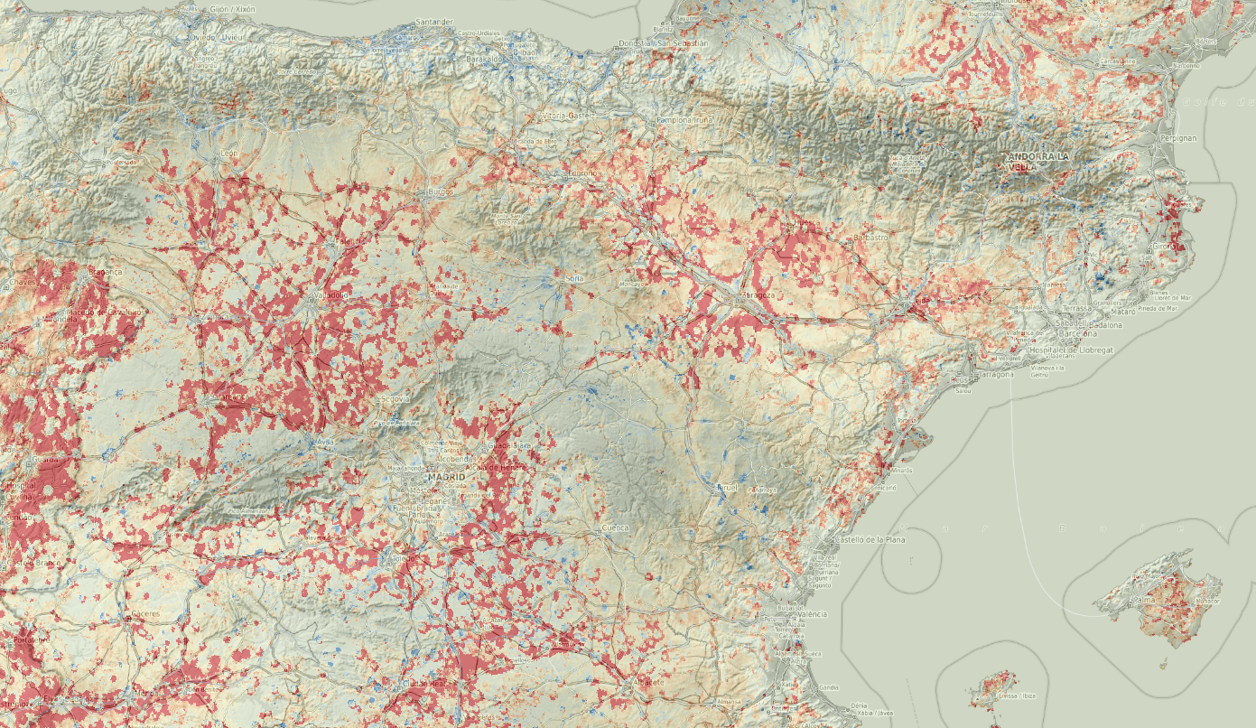

Figure 5.7: Trend map for mosquito distribution through time. Red color indicates increase in occurrence probability, blue color decrease.

5.7 Summary

In this chapter we demonstrate how to use occurrence-only records to map distribution of target species in spacetime. We again use Ensemble Machine Learning on training data overlaid in spacetime vs time-series of Night Light, vegetation, climatic images (years 2000–2021). The training data is limited to occurrence-only records and these are neither based on probability sampling nor a consistent in time. Probably more suited training data set would have been if for example meteorological stations across EU have recorded daily records of mosquito occurrence (0/1). Having a systematic records at dense and well distributed locations across Europe would be the perfect data set for this exercise, but even with using limited GBIF records we are able to produce relatively accurate maps of probability of occurrence.

Note that in the case study above, we could have also used time i.e. Year of observation as a covariate. If we would add Year as covariate to this training point data, then predictions would have probably shown that probability of occurrence is increasing significantly in the recent years. This does not necessarily has to match reality on the ground. Just because there are more records of the mosquito species for more recent years, that does not mean that the mosquito has appeared in recent years. In fact, if we would use Year as a covariate with this data, we would most likely introduce a bias in predictions (Syfert, Smith, & Coomes, 2013).

GBIF data is of course of limited use for SDM and comes with often misssing meta-information and has, of course, huge gaps (Marcer et al., 2022; Syfert et al., 2013). This does not means that also the analysis in this tutorial is flawed or should not be considered as trust-worthy; it only means that running any spatial analysis on GBIF data should be done with care and aiming at correct interpretation.

The simple alternative to derive (kernel) density maps of mosquitos for Europe would be to use the sparr::spattemp.density function:

st.f = occ[,c("decimalLongitude","decimalLatitude","Date","individualCount")]
st.f$individualCount = as.numeric(ifelse(is.na(st.f$individualCount), 1, st.f$individualCount))
coordinates(st.f) <- c("decimalLongitude", "decimalLatitude")
proj4string(st.f) <- CRS("+init=epsg:4326")
grid1d = readGDAL("./input/mask_5km.tif")
grid1d = as(grid1d, "SpatialPixelsDataFrame")
te = as.vector(grid1d@bbox)
#plot(grid1d)
mg_owin <- spatstat.geom::as.owin(data.frame(x = grid1d@coords[,1], y = grid1d@coords[,2], window = TRUE))
st.f_sp <- spTransform(st.f, grid1d@proj4string)
pp = ppp(x=st.f_sp@coords[,1], y=st.f_sp@coords[,2], marks=as.numeric(substr(st.f_sp$Date, 1, 4)), window = mg_owin)
## Warning messages:
#1: 41072 points were rejected as lying outside the specified window 
#2: data contain duplicated points
pp$n
## 13893
str(pp$marks)
## spacetime density ----
eu.stgrid = sparr::spattemp.density(pp, tt = pp$marks, tlim = c(2000,2022), sres=1569, verbose = TRUE)
## Calculating trivariate smooth...Done.
## Edge-correcting...Done.
## Conditioning on time...Done.
#plot(eu.stgrid, 2018)
dmap <- maptools::as.SpatialGridDataFrame.im(eu.stgrid$z[["2012"]])
summary(dmap$v*1e12)
plot(dmap)

The problem of usiong sparr::spattemp.density is that (a) it can be used only with occurrence only records, (b) it assumes that ALL or systematically sampled occurrences of the phenomena are available. If this is not the case, the function sparr::spattemp.density would also probably produce a biased estimate of the distribution of mosquitos through time.

Ensemble Machine Learning we used to generate predictions helps produce unbiased estimate of mosquito occurrences over Europe for a time-series of years. The disadvantages of using spatiotemporal ML are:

We are correlating the Earth Observation data with mosquito density, but mosquitos are dynamic and can not be sensed / seen from space, at least not at 1km resolution; we have to rely on correlation with environmental factors and this can explain only smaller part of variation;
We assume that the GBIF training points are representative for various environmental conditions, while in practice less training data is available for physically distant areas e.g. mountains (hence these training data can be considered to be censored);
Predictions produced in this example come with relatively high errors in extrapolation areas, so the predictions should be used together with the uncertainty maps;

5.8 Acknowledgments

This project has received funding from the European Union’s Horizon 2020 Research and innovation programme under grant agreement No 874850.

4 Spatiotemporal interpolation using Ensemble ML

6 Spatiotemporal prediction of Soil Organic Carbon