2 Spatial interpolation using Ensemble ML

You are reading the work-in-progress Spatial and spatiotemporal interpolation using Ensemble Machine Learning. This chapter is currently draft version, a peer-review publication is pending. You can find the polished first edition at https://opengeohub.github.io/spatial-prediction-eml/.

2.1 Spatial interpolation using ML and buffer distances to points

A relatively simple approach to interpolate values from point data using e.g. Random Forest is to use buffer distances to all points as covariates. We can here use the meuse dataset for testing (T. Hengl et al., 2018):

library(rgdal)
library(ranger)
library(raster)
library(plotKML)
demo(meuse, echo=FALSE)
grid.dist0 <- landmap::buffer.dist(meuse["zinc"], meuse.grid[1], 
                                   classes=as.factor(1:nrow(meuse)))

This creates 155 gridded maps i.e. one map per training point. These maps of distances can now be used to predict some target variable by running:

dn0 <- paste(names(grid.dist0), collapse="+")
fm0 <- as.formula(paste("zinc ~ ", dn0))
ov.zinc <- over(meuse["zinc"], grid.dist0)
rm.zinc <- cbind(meuse@data["zinc"], ov.zinc)
m.zinc <- ranger(fm0, rm.zinc, num.trees=150, seed=1)
m.zinc
#> Ranger result
#> 
#> Call:
#>  ranger(fm0, rm.zinc, num.trees = 150, seed = 1) 
#> 
#> Type:                             Regression 
#> Number of trees:                  150 
#> Sample size:                      155 
#> Number of independent variables:  155 
#> Mtry:                             12 
#> Target node size:                 5 
#> Variable importance mode:         none 
#> Splitrule:                        variance 
#> OOB prediction error (MSE):       67501.48 
#> R squared (OOB):                  0.4990359

Using this model we can generate and plot predictions using:

op <- par(oma=c(0,0,0,1), mar=c(0,0,4,3))
zinc.rfd <- predict(m.zinc, grid.dist0@data)$predictions
meuse.grid$zinc.rfd = zinc.rfd
plot(raster(meuse.grid["zinc.rfd"]), col=R_pal[["rainbow_75"]][4:20],
         main="Predictions RF on buffer distances", axes=FALSE, box=FALSE)
points(meuse, pch="+", cex=.8)
par(op)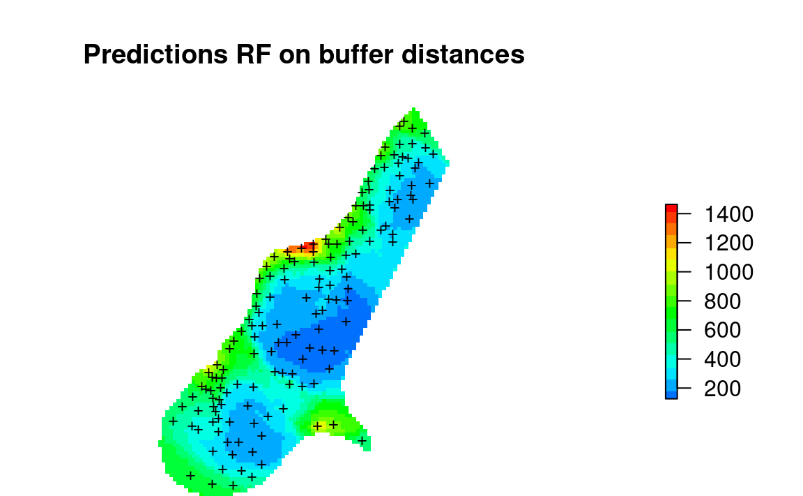

Figure 2.1: Values of Zinc predicted using only RF on buffer distances.

The resulting predictions produce patterns very much similar to what we would produce if we have used ordinary kriging or similar. Note however that for RFsp model: (1) we did not have to fit any variogram, (2) the model is in essence over- parameterized with basically more covariates than training points.

2.2 Spatial interpolation using ML and geographical distances to neighbors

Deriving buffer distances for all points is obviously not suitable for very large point datasets. Sekulić, Kilibarda, Heuvelink, Nikolić, & Bajat (2020) describe an alternative, a more scalable method that uses closest neighbors (and their values) as covariates to predict target variable. This can be implemented using the meteo package:

library(meteo)
#> Warning: replacing previous import 'caret::MAE' by 'DescTools::MAE' when
#> loading 'meteo'
#> Warning: replacing previous import 'caret::RMSE' by 'DescTools::RMSE' when
#> loading 'meteo'
nearest_obs <- meteo::near.obs(locations = meuse.grid, 
                               locations.x.y = c("x","y"), 
                               observations = meuse, observations.x.y=c("x","y"), 
                               zcol = "zinc", n.obs = 10, rm.dupl = TRUE)
#> Warning in if (class(knn1$nn.idx) != "integer") {: the condition has length > 1
#> and only the first element will be used
str(nearest_obs)
#> 'data.frame':    3103 obs. of  20 variables:
#>  $ dist1 : num  168.2 112 139.9 172 56.4 ...
#>  $ dist2 : num  204 165 164 173 127 ...
#>  $ dist3 : num  239 183 210 230 139 ...
#>  $ dist4 : num  282 268 246 241 265 ...
#>  $ dist5 : num  370 331 330 335 297 ...
#>  $ dist6 : num  407 355 370 380 306 ...
#>  $ dist7 : num  429 406 391 388 390 ...
#>  $ dist8 : num  504 448 473 472 393 ...
#>  $ dist9 : num  523 476 484 496 429 ...
#>  $ dist10: num  524 480 488 497 431 ...
#>  $ obs1  : num  1022 1022 1022 640 1022 ...
#>  $ obs2  : num  640 640 640 1022 1141 ...
#>  $ obs3  : num  1141 1141 1141 257 640 ...
#>  $ obs4  : num  257 257 257 1141 257 ...
#>  $ obs5  : num  346 346 346 346 346 346 346 346 346 346 ...
#>  $ obs6  : num  406 406 406 269 406 406 406 269 257 406 ...
#>  $ obs7  : num  269 269 269 406 269 ...
#>  $ obs8  : num  1096 1096 1096 281 1096 ...
#>  $ obs9  : num  347 347 347 347 504 347 347 279 269 504 ...
#>  $ obs10 : num  281 504 281 279 347 504 279 347 347 347 ...

which produces 20 grids showing assigned values from 1st to 10th neighbor and distances. We can plot values based on the first neighbor, which corresponds to using e.g. Voronoi polygons:

meuse.gridF = meuse.grid
meuse.gridF@data = nearest_obs
spplot(meuse.gridF[11])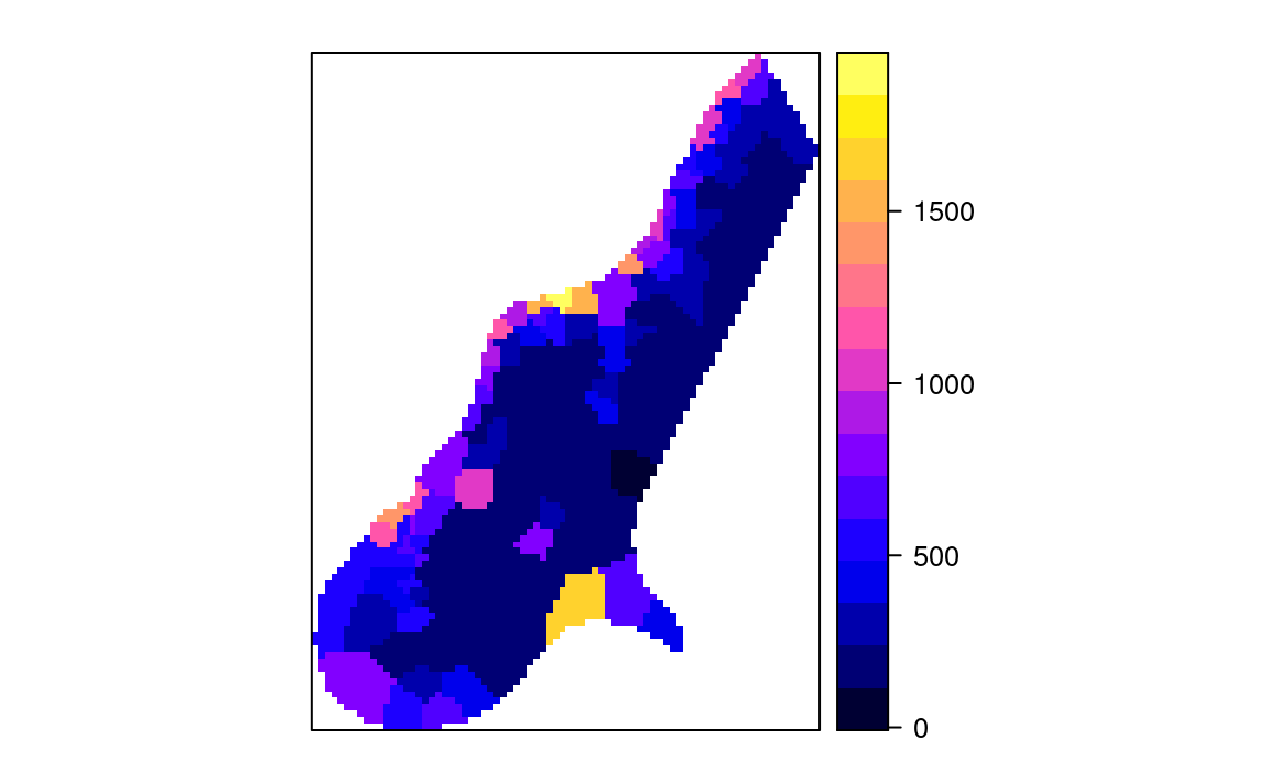

Figure 2.2: Values of first neighbor for meuse dataset.

Next, we can estimate the same values for training points, but this time we remove any duplicates using rm.dupl = TRUE:

## training points
nearest_obs.dev <- meteo::near.obs(locations = meuse, 
                                   locations.x.y = c("x","y"), 
                                   observations = meuse, 
                                   observations.x.y=c("x","y"), 
                                   zcol = "zinc", n.obs = 10, rm.dupl = TRUE)
#> Warning in if (class(knn1$nn.idx) != "integer") {: the condition has length > 1
#> and only the first element will be used
meuse@data <- cbind(meuse@data, nearest_obs.dev)

Finally, we can fit a model to predict values purely based on spatial autocorrelation between values (1st to 10th nearest neighbour):

fm.RFSI <- as.formula(paste("zinc ~ ", paste(paste0("dist", 1:10), collapse="+"), "+", paste(paste0("obs", 1:10), collapse="+")))
fm.RFSI
#> zinc ~ dist1 + dist2 + dist3 + dist4 + dist5 + dist6 + dist7 + 
#>     dist8 + dist9 + dist10 + obs1 + obs2 + obs3 + obs4 + obs5 + 
#>     obs6 + obs7 + obs8 + obs9 + obs10
rf_RFSI <- ranger(fm.RFSI, data=meuse@data, importance = "impurity", num.trees = 85, keep.inbag = TRUE)
rf_RFSI
#> Ranger result
#> 
#> Call:
#>  ranger(fm.RFSI, data = meuse@data, importance = "impurity", num.trees = 85,      keep.inbag = TRUE) 
#> 
#> Type:                             Regression 
#> Number of trees:                  85 
#> Sample size:                      155 
#> Number of independent variables:  20 
#> Mtry:                             4 
#> Target node size:                 5 
#> Variable importance mode:         impurity 
#> Splitrule:                        variance 
#> OOB prediction error (MSE):       65997.22 
#> R squared (OOB):                  0.5101999

To produce predictions we can run:

out = predict(rf_RFSI, meuse.gridF@data)
meuse.grid$zinc.rfsi = out$predictions
op <- par(oma=c(0,0,0,1), mar=c(0,0,4,3))
plot(raster(meuse.grid["zinc.rfsi"]), col=R_pal[["rainbow_75"]][4:20],
     main="Predictions RFSI", axes=FALSE, box=FALSE)
points(meuse, pch="+", cex=.8)
par(op)
#dev.off()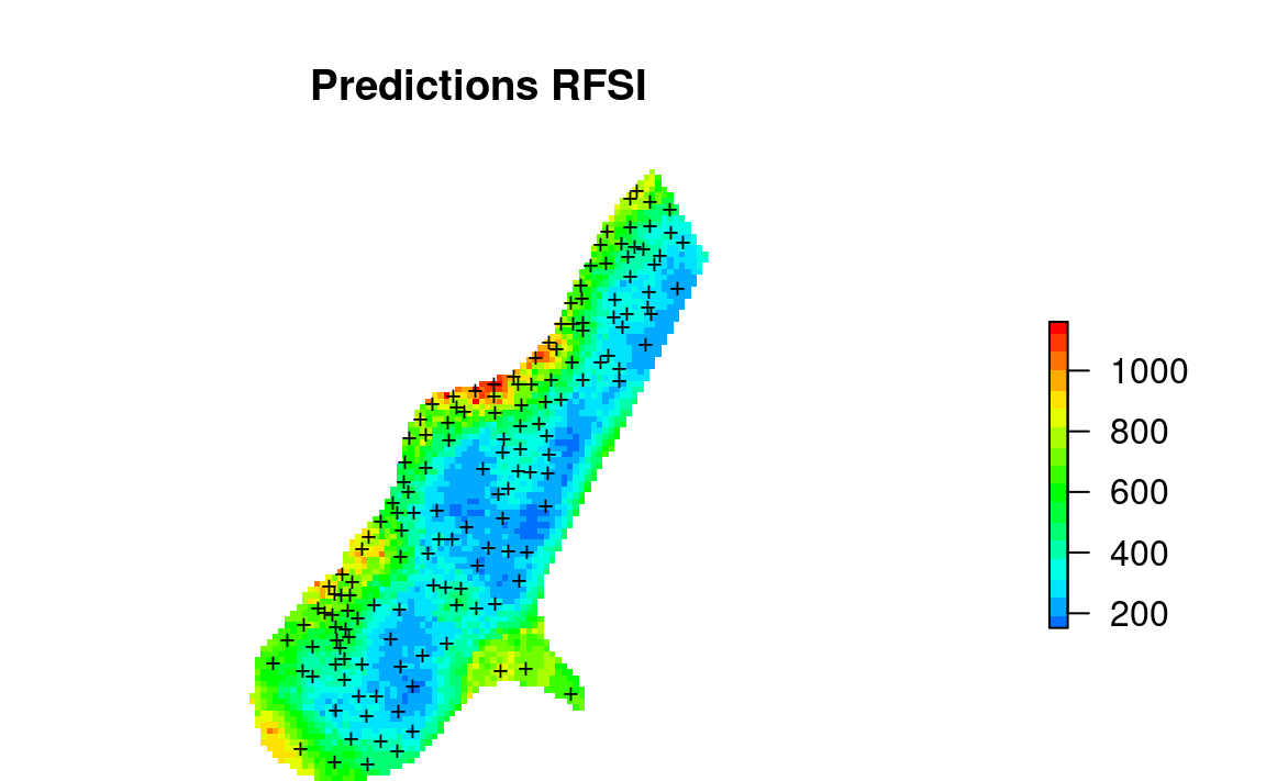

Figure 2.3: Values of first neighbor for meuse dataset.

In summary, based on the Figs. 2.1 and 2.3, we can conclude that predictions produced using nearest neighbors (Fig. 2.3) show quite different patterns than predictions based on buffer distances (Fig. 2.1). The method by Sekulić et al. (2020) (Random Forest Spatial Interpolation) RFSI is probably more interesting for general applications as it could be also added to spatiotemporal data problems. It also reflects closely idea of using spatial autocorrelation of values as used in kriging since both values of neighbors and distances to neighbors are used as covariates. On the other hand, RFSI seem to produce predictions that contain also short range variability (more noisy) and as such predictions might appear to look more like geostatistical simulations.

2.3 Interpolation of numeric values using spatial regression

We load the packages that will be used in this tutorial:

library(landmap)
library(rgdal)
library(geoR)
#> --------------------------------------------------------------
#>  Analysis of Geostatistical Data
#>  For an Introduction to geoR go to http://www.leg.ufpr.br/geoR
#>  geoR version 1.8-1 (built on 2020-02-08) is now loaded
#> --------------------------------------------------------------
library(plotKML)
library(raster)
library(glmnet)
library(xgboost)
library(kernlab)
#> 
#> Attaching package: 'kernlab'
#> The following objects are masked from 'package:raster':
#> 
#>     buffer, rotated
library(deepnet)
library(forestError)
library(mlr)

For testing we use meuse data set. We can fit a 2D model to interpolate zinc concentration based on sampling points, distance to the river and flooding frequency maps by using:

demo(meuse, echo=FALSE)
m <- train.spLearner(meuse["zinc"], covariates=meuse.grid[,c("dist","ffreq")], 
                     lambda = 1, parallel=FALSE)
#> # weights:  103
#> initial  value 51302358.935975 
#> final  value 19491244.345324 
#> converged
#> # weights:  103
#> initial  value 45220763.375836 
#> final  value 16169762.129496 
#> converged
#> # weights:  103
#> initial  value 50723533.722266 
#> final  value 18557431.400000 
#> converged
#> # weights:  103
#> initial  value 52179393.837805 
#> final  value 19673925.525180 
#> converged
#> # weights:  103
#> initial  value 48966129.905012 
#> final  value 19237393.850000 
#> converged
#> # weights:  103
#> initial  value 50327217.343373 
#> final  value 19238858.992857 
#> converged
#> # weights:  103
#> initial  value 50106999.812372 
#> final  value 19072846.949640 
#> converged
#> # weights:  103
#> initial  value 48513819.381025 
#> final  value 18339886.345324 
#> converged
#> # weights:  103
#> initial  value 48861791.596477 
#> final  value 18454493.171429 
#> converged
#> # weights:  103
#> initial  value 48476787.002316 
#> final  value 18430903.600000 
#> converged
#> # weights:  103
#> initial  value 54933965.304156 
#> final  value 20750447.509677 
#> converged

This runs number of steps including derivation of geographical distances (Møller, Beucher, Pouladi, & Greve, 2020), derivation of principal components (to make sure all features are numeric and complete), fitting of variogram using the geoR package (Diggle & Ribeiro Jr, 2007), spatial overlay, training of individual learners and training of the super learner. In principle, the only parameter we need to set manually in the train.spLearner is the lambda = 1 which is required to estimate variogram: in this case the target variable is log-normally distributed, and hence the geoR package needs the transformation parameter set at lambda = 1.

Note that the default meta-learner in train.spLearner is a linear model from five independently fitted learners c("regr.ranger", "regr.xgboost", "regr.ksvm", "regr.nnet", "regr.cvglmnet"). We can check the success of training based on the 5-fold spatial Cross-Validation using:

summary(m@spModel$learner.model$super.model$learner.model)
#> 
#> Call:
#> stats::lm(formula = f, data = d)
#> 
#> Residuals:
#>     Min      1Q  Median      3Q     Max 
#> -470.94  -97.78  -15.73   64.59 1049.38 
#> 
#> Coefficients:
#>                Estimate Std. Error t value Pr(>|t|)    
#> (Intercept)   2146.8982   968.9798   2.216 0.028234 *  
#> regr.ranger      0.6822     0.1912   3.569 0.000483 ***
#> regr.xgboost     0.5249     0.4071   1.289 0.199244    
#> regr.nnet       -4.5017     2.0482  -2.198 0.029499 *  
#> regr.ksvm        0.4241     0.2148   1.975 0.050145 .  
#> regr.cvglmnet   -0.2757     0.1648  -1.673 0.096441 .  
#> ---
#> Signif. codes:  0 '***' 0.001 '**' 0.01 '*' 0.05 '.' 0.1 ' ' 1
#> 
#> Residual standard error: 199.9 on 149 degrees of freedom
#> Multiple R-squared:  0.7132, Adjusted R-squared:  0.7036 
#> F-statistic:  74.1 on 5 and 149 DF,  p-value: < 2.2e-16

Which shows that the model explains about 65% of variability in target variable and that regr.ranger learner (Wright & Ziegler, 2017) is the strongest learner. Average mapping error RMSE = 213, hence the models is somewhat more accurate than if we only used buffer distances.

To predict values at all grids we use:

meuse.y <- predict(m)
#> Predicting values using 'getStackedBaseLearnerPredictions'...TRUE
#> Deriving model errors using forestError package...TRUE

Note that, by default, we will predict two outputs:

Mean prediction: i.e. the best unbiased prediction of response;
Prediction errors: usually predicted as lower and upper 67% quantiles (1 std.) based on the forestError (Lu & Hardin, 2021);

If not otherwise specified, derivation of the prediction error (Root Mean Square Prediction Error), bias and lower and upper prediction intervals is implemented by default via the forestError algorithm. The method is explained in detail in Lu & Hardin (2021).

We could also produce the prediction intervals by using the quantreg Random Forest algorithm (Meinshausen, 2006) as implemented in the ranger package, or as a standard deviation of the bootstraped models, although using the method by Lu & Hardin (2021) is recommended.

To determine the prediction errors without drastically increasing computing time, we basically fit an independent random forest model using the five base-learners with setting quantreg = TRUE:

zinc ~ regr.ranger + regr.xgboost + regr.nnet + regr.ksvm + regr.cvglmnet

The prediction error methods are non-parameteric and users can choose any probability in the output via the quantiles argument. For example, the default quantiles are set to produce prediction intervals for the .682 range, which is the 1-standard-deviation range in the case of a Gaussian distribution. Deriving prediction errors, however, can be come computational for large number of features and trees in the random forest, so have in mind that EML comes with exponentially increased computing time.

We can plot the predictions and prediction errors next to each other by using:

par(mfrow=c(1,2), oma=c(0,0,0,1), mar=c(0,0,4,3))
plot(raster(meuse.y$pred["response"]), col=R_pal[["rainbow_75"]][4:20],
     main="Predictions spLearner", axes=FALSE, box=FALSE)
points(meuse, pch="+", cex=.8)
plot(raster(meuse.y$pred["model.error"]), col=rev(bpy.colors()),
     main="Prediction errors", axes=FALSE, box=FALSE)
points(meuse, pch="+", cex=.8)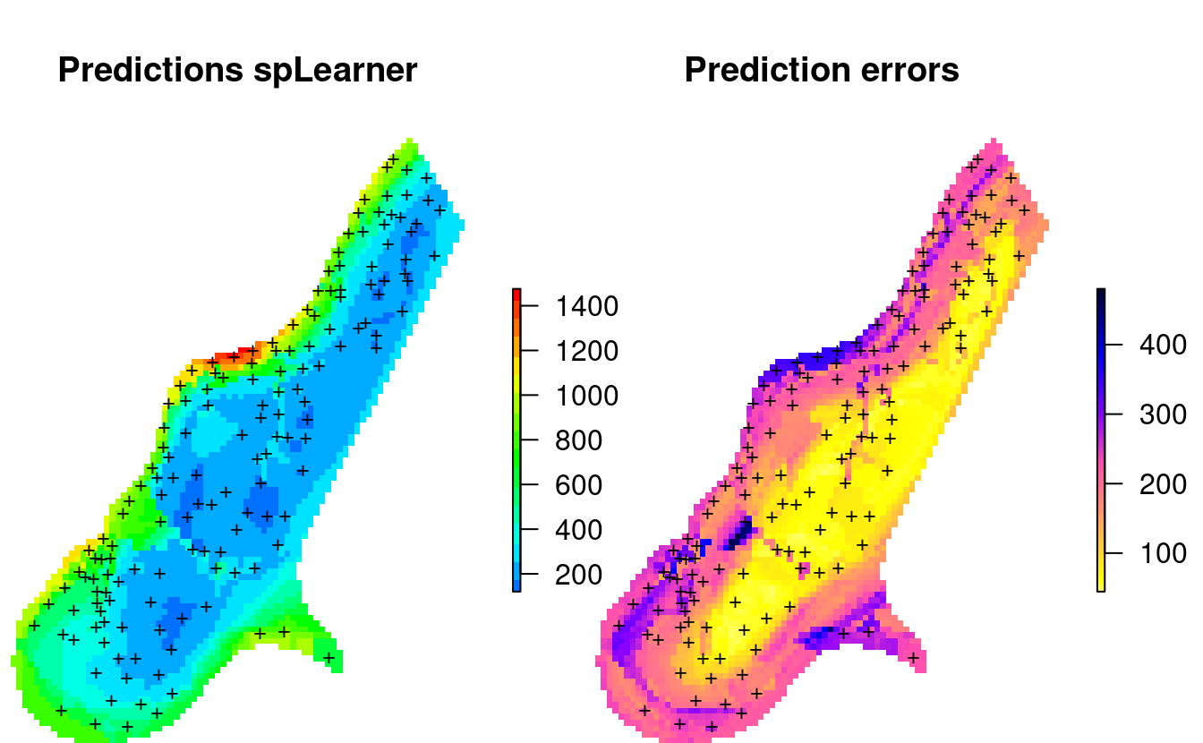

Figure 2.4: Predicted zinc content based on meuse data set.

This shows that the prediction errors (right plot) are the highest:

where the model is getting further away from the training points (spatial extrapolation),
where individual points with high values can not be explained by covariates,
where measured values of the response variable are in general high,

We can also plot the lower and upper prediction intervals for the .682 probability range using:

pts = list("sp.points", meuse, pch = "+", col="black")
spplot(meuse.y$pred[,c("q.lwr","q.upr")], col.regions=R_pal[["rainbow_75"]][4:20],
       sp.layout = list(pts),
       main="Prediction intervals (alpha = 0.318)")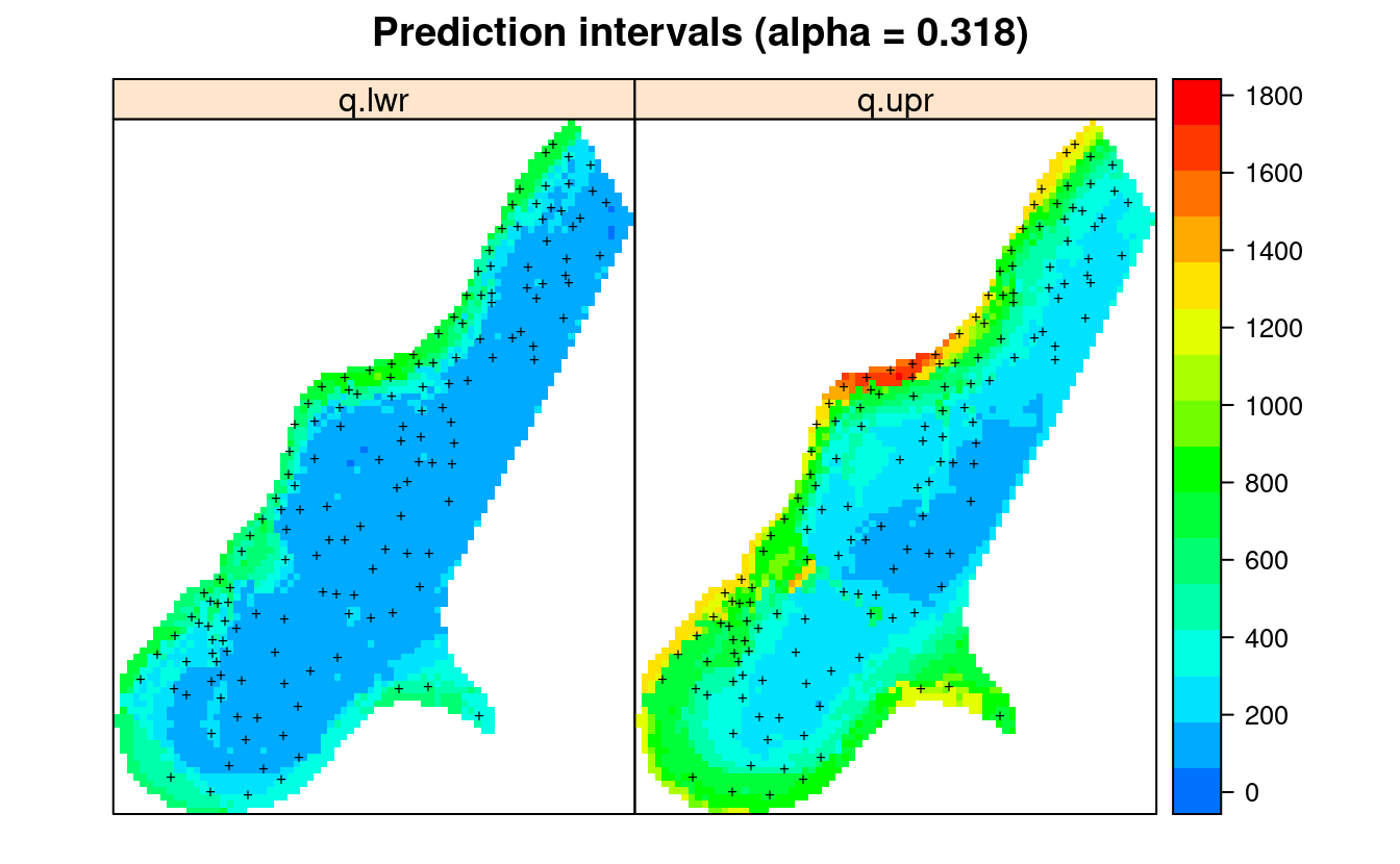

Figure 2.5: Lower (q.lwr) and upper (q.upr) prediction intervals for zinc content based on meuse data set.

2.4 Model fine-tuning and feature selection

The function tune.spLearner can be used to further optimize spLearner object by:

fine-tuning model parameters, especially the ranger mtry and XGBoost parameters,
reduce number of features by running feature selection via the mlr::makeFeatSelWrapper function,

The package landmap currently requires that two base learners used include regr.ranger and regr.xgboost, and that there are at least 3 base learners in total. The model from above can be optimized using:

m0 <- tune.spLearner(m, xg.skip=TRUE, parallel=FALSE)

which reports RMSE for different mtry and reports which features have been left and which removed. Note that we turn off the fine-tuning of XGboost using xg.skip = TRUE as it takes at the order of magnitude more time. In summary, in this specific case, the fine-tuned model is not much more accurate, but it comes with the less features:

str(m0@spModel$features)

chr [1:11] "PC2" "PC3" "PC4" "rX_0" "rY_0" "rY_0.2" "rX_0.5" "rY_1" "rY_1.4" "rY_2.9" "rY_3.1"

summary(m0@spModel$learner.model$super.model$learner.model)

Residuals:
    Min      1Q  Median      3Q     Max 
-404.09 -139.03  -42.05   64.69 1336.47 

Coefficients:
                Estimate Std. Error t value Pr(>|t|)   
(Intercept)   2091.87119  661.70995   3.161  0.00190 **
regr.ranger      0.14278    0.24177   0.591  0.55570   
regr.xgboost     0.92283    0.53131   1.737  0.08448 . 
regr.nnet       -4.34961    1.38703  -3.136  0.00206 **
regr.ksvm        0.66590    0.25027   2.661  0.00865 **
regr.cvglmnet   -0.08703    0.13808  -0.630  0.52944   
---
Signif. codes:  0 ‘***’ 0.001 ‘**’ 0.01 ‘*’ 0.05 ‘.’ 0.1 ‘ ’ 1

Residual standard error: 245.2 on 149 degrees of freedom
Multiple R-squared:  0.5683,    Adjusted R-squared:  0.5538 
F-statistic: 39.23 on 5 and 149 DF,  p-value: < 2.2e-16

Note that fine-tuning and feature selection can be quite computational and it is highly recommended to start with smaller subsets of data and then measure processing time. Note that the function mlr::makeFeatSelWrapper can result in errors if the covariates have a low variance or follow a zero-inflated distribution. Reducing the number of features via feature selection and fine-tuning of the Random Forest mtry and XGboost parameters, however, can result in significantly higher prediction speed and can also help improve accuracy.

2.5 Estimation of prediction intervals

We can also print the lower and upper prediction interval for every location using e.g.:

sp::over(meuse[1,], meuse.y$pred)
#>   response model.error model.bias    q.lwr    q.upr
#> 1 999.8759    214.1839   27.39722 749.5775 1289.188

where q.lwr is the lower and q.upr is the 68% probability upper quantile value. This shows that the 68% probability interval for the location x=181072, y=333611 is about 734–1241 which means that the prediction error (±1 s.d.), at that location, is about 250. Compare with the actual value sampled at that location:

meuse@data[1,"zinc"]
#> [1] 1022

The average prediction error for the whole area is:

summary(meuse.y$pred$model.error)
#>    Min. 1st Qu.  Median    Mean 3rd Qu.    Max. 
#>   44.63   77.04  167.69  159.58  215.06  480.11

which is somewhat lower than the RMSE derived by cross-validation, but this is also because most of the predicted values are in fact low (skewed distribution), and EML seems not have many problems predicting low values.

Note also, from the example above, if we refit a model using exactly the same settings we might get somewhat different maps and different values. This is to be expected as the number of training points and covariates is low, the stacking is done by using (random) 5-fold Cross-validation, and hence results will always be slightly different. The resulting models and maps, however, should not be significantly different as this would indicate that the Ensemble ML is unstable. In the case of larger datasets (≫1000 points), differences between predictions should become less and less visible.

2.6 Predictions using log-transformed target variable

If the purpose of spatial prediction to make a more accurate predictions of low(er) values of the response, then we can train a model with the transformed variable:

meuse$log.zinc = log1p(meuse$zinc)
m2 <- train.spLearner(meuse["log.zinc"], covariates=meuse.grid[,c("dist","ffreq")], parallel=FALSE)
#> # weights:  103
#> initial  value 4998.882579 
#> final  value 73.222851 
#> converged
#> # weights:  103
#> initial  value 5683.969732 
#> final  value 68.561330 
#> converged
#> # weights:  103
#> initial  value 4834.044628 
#> final  value 68.897172 
#> converged
#> # weights:  103
#> initial  value 5706.570659 
#> final  value 72.649748 
#> converged
#> # weights:  103
#> initial  value 2349.857144 
#> final  value 73.103072 
#> converged
#> # weights:  103
#> initial  value 6184.275769 
#> final  value 74.169414 
#> converged
#> # weights:  103
#> initial  value 4451.463365 
#> final  value 69.440176 
#> converged
#> # weights:  103
#> initial  value 4852.414287 
#> final  value 72.774801 
#> converged
#> # weights:  103
#> initial  value 5902.359343 
#> final  value 72.079999 
#> converged
#> # weights:  103
#> initial  value 6689.386512 
#> final  value 72.803948 
#> converged
#> # weights:  103
#> initial  value 5607.506170 
#> final  value 79.790191 
#> converged

The summary model will usually have a somewhat higher R-square, but the best learners should stay about the same:

summary(m2@spModel$learner.model$super.model$learner.model)
#> 
#> Call:
#> stats::lm(formula = f, data = d)
#> 
#> Residuals:
#>      Min       1Q   Median       3Q      Max 
#> -1.00361 -0.18873 -0.05022  0.14092  1.41474 
#> 
#> Coefficients:
#>               Estimate Std. Error t value Pr(>|t|)    
#> (Intercept)   25.75549   10.10511   2.549 0.011822 *  
#> regr.ranger    0.74984    0.19969   3.755 0.000248 ***
#> regr.xgboost   0.31617    0.33255   0.951 0.343264    
#> regr.nnet     -4.44329    1.70769  -2.602 0.010206 *  
#> regr.ksvm      0.28476    0.19541   1.457 0.147146    
#> regr.cvglmnet -0.07384    0.15905  -0.464 0.643137    
#> ---
#> Signif. codes:  0 '***' 0.001 '**' 0.01 '*' 0.05 '.' 0.1 ' ' 1
#> 
#> Residual standard error: 0.3574 on 149 degrees of freedom
#> Multiple R-squared:  0.7615, Adjusted R-squared:  0.7535 
#> F-statistic: 95.14 on 5 and 149 DF,  p-value: < 2.2e-16

We can next predict and then back-transform the values:

meuse.y2 <- predict(m2)
#> Predicting values using 'getStackedBaseLearnerPredictions'...TRUE
#> Deriving model errors using forestError package...TRUE
## back-transform:
meuse.y2$pred$response.t = expm1(meuse.y2$pred$response)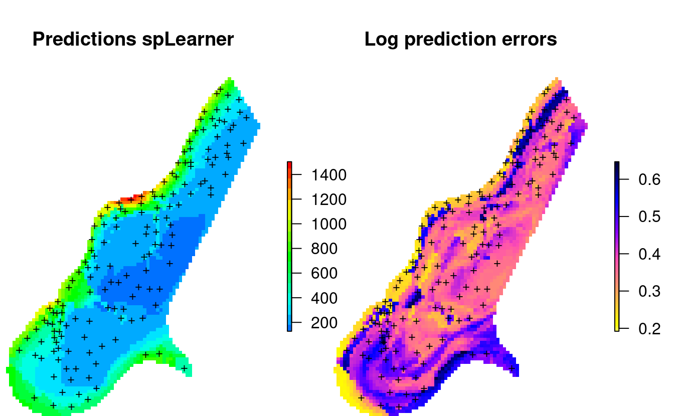

Figure 2.6: Predicted zinc content based on meuse data set after log-transformation.

The predictions (Figs. 2.4 and 2.6) show similar patterns but the prediction error maps are quite different in this case. Nevertheless, the problem areas seem to match in both maps (see Figs. 2.4 and 2.6 right part). If we compare distributions of two predictions we can also see that the predictions do not differ much:

library(ggridges)
library(viridis)
#> Loading required package: viridisLite
library(ggplot2)
#> 
#> Attaching package: 'ggplot2'
#> The following object is masked from 'package:kernlab':
#> 
#>     alpha
zinc.df = data.frame(zinc=c(sp::over(meuse, meuse.y$pred["response"])[,1], 
                            sp::over(meuse, meuse.y2$pred["response.t"])[,1],
                            meuse$zinc
))
zinc.df$type = as.vector(sapply(c("predicted", "log.predicted", "observed"), function(i){rep(i, nrow(meuse))}))
ggplot(zinc.df, aes(x = zinc, y = type, fill = ..x..)) +
  geom_density_ridges_gradient(scale = 0.95, rel_min_height = 0.01, gradient_lwd = 1.) +
  scale_x_continuous(expand = c(0.01, 0)) +
  ## scale_x_continuous(trans='log2') +
  scale_y_discrete(expand = c(0.01, 0.01)) +
  scale_fill_viridis(name = "Zinc", option = "C") +
  labs(title = "Distributions comparison") +
  theme_ridges(font_size = 13, grid = TRUE) + theme(axis.title.y = element_blank())
#> Picking joint bandwidth of 110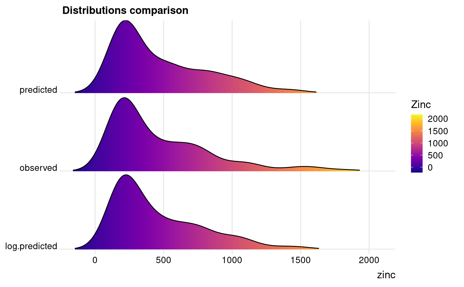

Figure 2.7: Difference in distributions observed and predicted.

The observed very high values are somewhat smoothed out but the median value is about the same, hence we can conclude that the two EML models predict the target variable without a bias. To estimate the prediction intervals using the log-transformed variable we can use:

x = sp::over(meuse[1,], meuse.y2$pred)
expm1(x$q.lwr); expm1(x$q.upr)
#> [1] 837.8133
#> [1] 1638.359

Note that the log-transformation is not needed for a non-linear learner such ranger and/or Xgboost, but it is often a good idea if the focus of prediction is to get a better accuracy for lower values (Tomislav Hengl et al., 2021). For example, if the objective of spatial interpolation is to map soil nutrient deficiencies, then log-transformation is a good idea as it will produce slightly better accuracy for lower values.

Another advantage of using log-transformation for log-normal variables is that the prediction intervals would most likely be symmetric, so that derivation of prediction error (±1 s.d.) can be derived by:

pe = (q.upr - q.lwr)/2

2.7 Spatial prediction of soil types (factor-variable)

Ensemble Machine Learning can also be used to interpolate factor type variables e.g. soil types. This is an example with the Ebergotzen dataset available from the package plotKML (T. Hengl et al., 2015):

library(plotKML)
data(eberg_grid)
gridded(eberg_grid) <- ~x+y
proj4string(eberg_grid) <- CRS("+init=epsg:31467")
data(eberg)
coordinates(eberg) <- ~X+Y
proj4string(eberg) <- CRS("+init=epsg:31467")
summary(eberg$TAXGRSC)
#>     Auenboden     Braunerde          Gley         HMoor    Kolluvisol 
#>            71           790            86             1           186 
#>          Moor Parabraunerde  Pararendzina       Pelosol    Pseudogley 
#>             1           704           215           252           487 
#>        Ranker       Regosol      Rendzina          NA's 
#>            20           376            23           458

In this case the target variable is TAXGRSC soil types based on the German soil classification system. This changes the modeling problem from regression to classification. We recommend using the following learners here:

sl.c <- c("classif.ranger", "classif.xgboost", "classif.nnTrain")

The model training and prediction however looks the same as for the regression:

X <- eberg_grid[c("PRMGEO6","DEMSRT6","TWISRT6","TIRAST6")]
if(!exists("mF")){
  mF <- train.spLearner(eberg["TAXGRSC"], covariates=X, parallel=FALSE)
}
#> Converting PRMGEO6 to indicators...
#> Converting covariates to principal components...
#> Deriving oblique coordinates...TRUE
#> Subsetting observations to 79% complete cases...TRUE
#> Skipping variogram modeling...TRUE
#> Estimating block size ID for spatial Cross Validation...TRUE
#> Using learners: classif.ranger, classif.xgboost, classif.nnTrain...TRUE
#> Fitting a spatial learner using 'mlr::makeClassifTask'...TRUE

To generate predictions we use:

if(!exists("TAXGRSC")){
  TAXGRSC <- predict(mF)
}
#> Predicting values using 'getStackedBaseLearnerPredictions'...TRUE
#> Deriving model errors using sd of sign. learners...TRUE

2.8 Classification accuracy

By default landmap package will predict both hard classes and probabilities per class. We can check the average accuracy of classification by using:

newdata = mF@vgmModel$observations@data
sel.e = complete.cases(newdata[,mF@spModel$features])
newdata = newdata[sel.e, mF@spModel$features]
pred = predict(mF@spModel, newdata=newdata)
pred$data$truth = mF@vgmModel$observations@data[sel.e, "TAXGRSC"]
print(calculateConfusionMatrix(pred))
#>                predicted
#> true            Auenboden Braunerde Gley Kolluvisol Parabraunerde Pararendzina
#>   Auenboden            34         6    0          0             5            0
#>   Braunerde             0       623    0          1            17            7
#>   Gley                  4         9   38          3             9            0
#>   Kolluvisol            0        13    1         99            17            1
#>   Parabraunerde         0        34    0          3           460            0
#>   Pararendzina          0        19    0          0             3          147
#>   Pelosol               0        11    0          1             1            2
#>   Pseudogley            0        54    2          4            24            3
#>   Ranker                0        10    0          0             6            0
#>   Regosol               0        66    0          0            10            1
#>   Rendzina              0         2    0          0             0            0
#>   -err.-                4       224    3         12            92           14
#>                predicted
#> true            Pelosol Pseudogley Ranker Regosol Rendzina -err.-
#>   Auenboden           0          3      0       0        0     14
#>   Braunerde           9          5      0       6        1     46
#>   Gley                0          5      0       0        0     30
#>   Kolluvisol          1          3      0       3        0     39
#>   Parabraunerde       2         10      0       4        0     53
#>   Pararendzina        6          1      0       0        0     29
#>   Pelosol           157          4      0       1        0     20
#>   Pseudogley          4        307      0      13        0    104
#>   Ranker              1          0      0       0        0     17
#>   Regosol             4         12      0     220        0     93
#>   Rendzina            0          0      0       0       20      2
#>   -err.-             27         43      0      27        1    447

which shows that about 25% of classes are miss-classified and the classification confusion is especially high for the Braunerde class. Note the result above is based only on the internal training. Normally one should repeat the process several times using 5-fold or similar (i.e. fit EML, predict errors using resampled values only, then repeat).

Predicted probabilities, however, are more interesting because they also show where EML possibly has problems and which are the transition zones between multiple classes:

plot(stack(TAXGRSC$pred[grep("prob.", names(TAXGRSC$pred))]),
     col=SAGA_pal[["SG_COLORS_YELLOW_RED"]], zlim=c(0,1))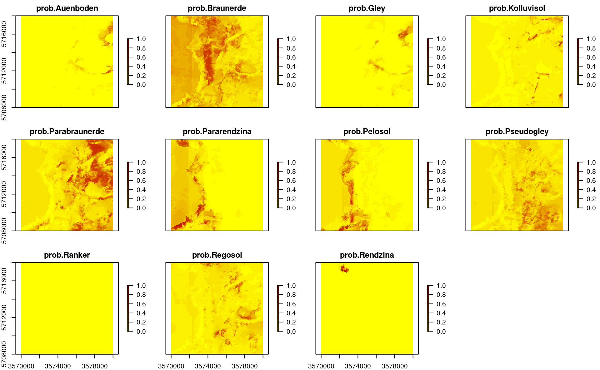

Figure 2.8: Predicted soil types based on EML.

The maps show that also in this case geographical distances play a role, but overall, the features (DTM derivatives and parnt material) seem to be most important.

In addition to map of probabilities per class, we have also derived errors per probability, which in this case can be computed as the standard deviation between probabilities produced by individual learners (note: for classification problems techniques such as quantreg random forest currently do not exist):

plot(stack(TAXGRSC$pred[grep("error.", names(TAXGRSC$pred))]),
     col=SAGA_pal[["SG_COLORS_YELLOW_BLUE"]], zlim=c(0,0.45))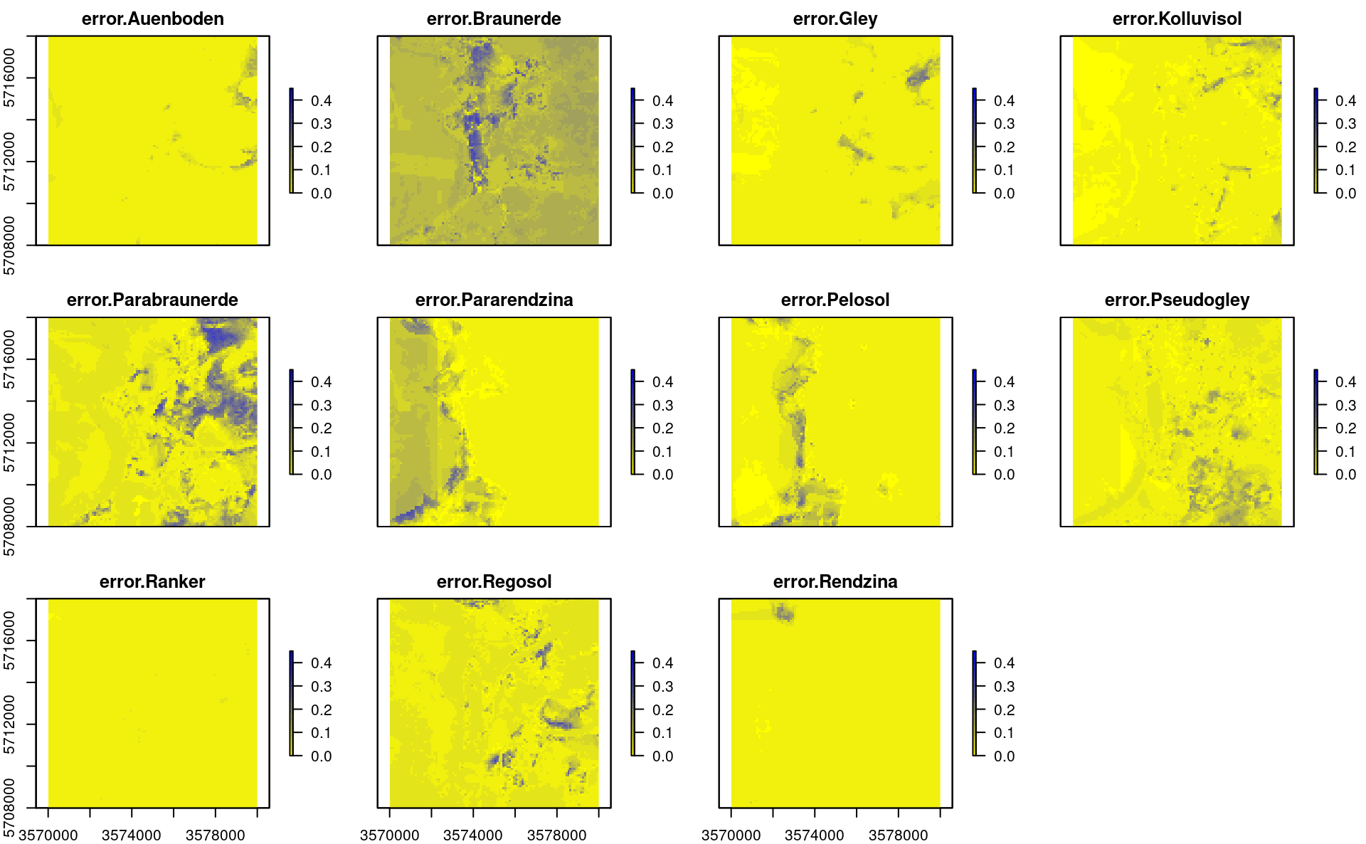

Figure 2.9: Predicted errors per soil types based on s.d. between individual learners.

In probability space, instead of using RMSE or similar measures, it is often recommended to use the measures such as the log-loss which correctly quantifies the difference between the observed and predicted probability. As a rule of thumb, log-loss values above 0.35 indicate poor accuracy of predictions, but the threshold number for critically low log-loss also depends on the number of classes. In the plot above we can note that, in general, the average error in maps is relatively low e.g. about 0.07:

summary(TAXGRSC$pred$error.Parabraunerde)
#>     Min.  1st Qu.   Median     Mean  3rd Qu.     Max. 
#> 0.001558 0.029074 0.041220 0.066121 0.064179 0.339019

but there are still many pixels where confusion between classes and prediction errors are high. Recommended strategy to improve this map is to generate a sampling plan using the average prediction error and/or Confusion Index map, then collect new observations & measurements and refit the prediction models.

1 Introduction to spatial and spatiotemporal data

3 Spatial interpolation in 3D using Ensemble ML