6 Spatiotemporal prediction of Soil Organic Carbon

You are reading the work-in-progress Spatial and spatiotemporal interpolation using Ensemble Machine Learning. This chapter is currently draft version, a peer-review publication is pending. You can find the polished first edition at https://opengeohub.github.io/spatial-prediction-eml/.

Prepared by: Tom Hengl (OpenGeoHub), Tania Maxwell (Department of Zoology, University of Cambridge) and Leandro Parente (OpenGeoHub)

6.1 Soil organic carbon: global mangrove forests

Soil organic carbon (SOC) is one of the most important soil properties of interest for Earth System and Life sciences, and various environmental monitoring projects. Soil organic carbon is symbol of healthy soil and also if we increase carbon sequestration from atmosphere to soil, we could potentially could help mitigate global warming effects of GHG (Lal, 2022).

In this tutorial we explain how soil samples (points) can be used in combination with time-series of Earth Observation and climatic data to map SOC stocks and potentially also changes in SOC through time. For this we use the Global compilation of soil organic carbon samples for world mangrove forest (Sanderman et al., 2018), which we combine with other soil samples from various project (resulting in a total of +12,000 samples). We overlay the points in space and time vs dynamic time-series EO data and some static covariates. We then fit spatiotemporal Ensemble Machine Learning model and generate predictions for 30×30km tiles (about 1459 tiles with mangrove mask).

The analysis was run for the needs of the project State of the World’s Mangroves 2022 run by the Global Mangrove Alliance (Leal & Spalding, 2022). The objectives of this work are:

Provide best unbiased estimate of SOC stocks at 30-m spatial resolution for recent time-period (2020–2021) with uncertainty,
Test if predictions in Sanderman et al. (2018) can be improved by using spatiotemporal EML vs RF only,
Provide open access to data and computational steps and regularly update predictions using new training points, new covariates and models,

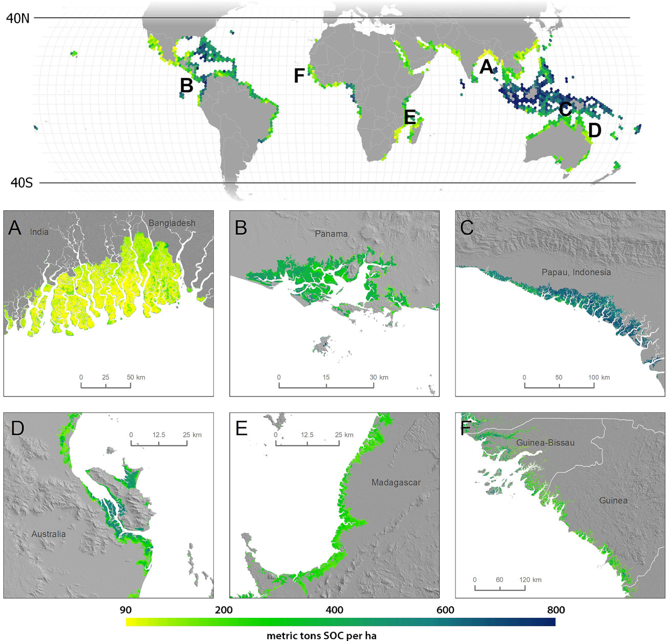
Figure 6.1: Global predictions of SOC stock for 0–1 m for mangroves based on Sanderman et al. (2018).

6.2 Predictive mapping of soil organic carbon stocks

In principle, there are at least three (3) ways to map soil organic carbon stocks (T. Hengl & MacMillan, 2019):

Estimate SOC stocks (t/ha) then produce 2D model and predict,
Model SOC density (kg/m3) in 3D, then aggregate to fixed depths,
Model SOC %, bulk density and coarse fragments separately in 3D, then aggregate to SOC density and to fixed depths,

Choice between the three is often determined by the project objectives and availability of data. For example, if most of point measurements are from top-soil as in LUCAS soil (Orgiazzi, Ballabio, Panagos, Jones, & Fernández-Ugalde, 2018), then probably makes most sense to estimate first SOC stocks in t/ha at point locations, then map 2D distribution of SOC stocks. If majority of data is collected at irregular depths (soil horizons) then it is probably more sensible to use 3D modeling. If for majority of point data bulk density is unknown (which is often the case), then it is probably most sensible to use approach #3 i.e. model SOC content (%), bulk density and coarse fragments independently, then combine values.

Formulas with example of how to derive SOC stocks (t/ha) (Tomislav Hengl et al., 2014) are shown in the scheme below.

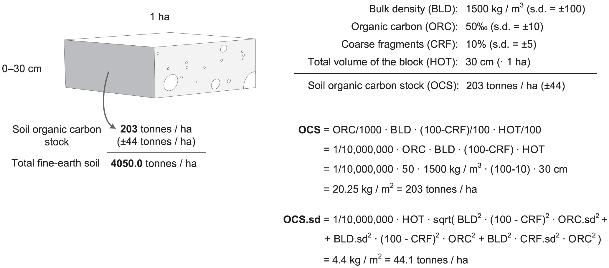
Example of how total soil organic carbon stock (OCS) and its propagated error can be estimated for a given volume of soil using organic carbon content (ORC), bulk density (BLD), thickness of horizon (HOT), and percentage of coarse fragments (CRF). Source: https://doi.org/10.1371/journal.pone.0105992.g006

Figure 6.2: Example of how total soil organic carbon stock (OCS) and its propagated error can be estimated for a given volume of soil using organic carbon content (ORC), bulk density (BLD), thickness of horizon (HOT), and percentage of coarse fragments (CRF). Source: https://doi.org/10.1371/journal.pone.0105992.g006

6.3 Training data

We use a compilation of soil samples analyzed in laboratory and digitized primarily from various literature. The original set from Sanderman et al. (2018) was extended with additional samples digitized from more recent literature sources by The Nature Conservancy and University of Cambridge. The analysis-ready data set overlaid vs time-series of EO covariates (regression-matrix) can be loaded by:

rms.df = readRDS("./input/world.mangroves_soil.carbon_rm.rds")
sel.db = rms.df$source_db %in% c("MangrovesDB","TNC_mangroves_2022","CSIRO_NatSoil","PRONASOLOS")
dim(rms.df)
#> [1] 11992   225

Note that, unlike the training points used in Sanderman et al. (2018), some of the points also fall in non-mangrove areas. This was done on purpose to help model transition zones from mangroves to non-mangrove areas.

We can start by getting acquainted with this dataset. First, we can check general distribution of values of SOC content (g/kg) vs soil depth:

openair::scatterPlot(rms.df[sel.db,], x = "hzn_depth", y = "oc", method = "hexbin", col = "increment", type = "source_db", log.x = TRUE, log.y = TRUE, xlab="Depth", ylab="SOC [g/kg]")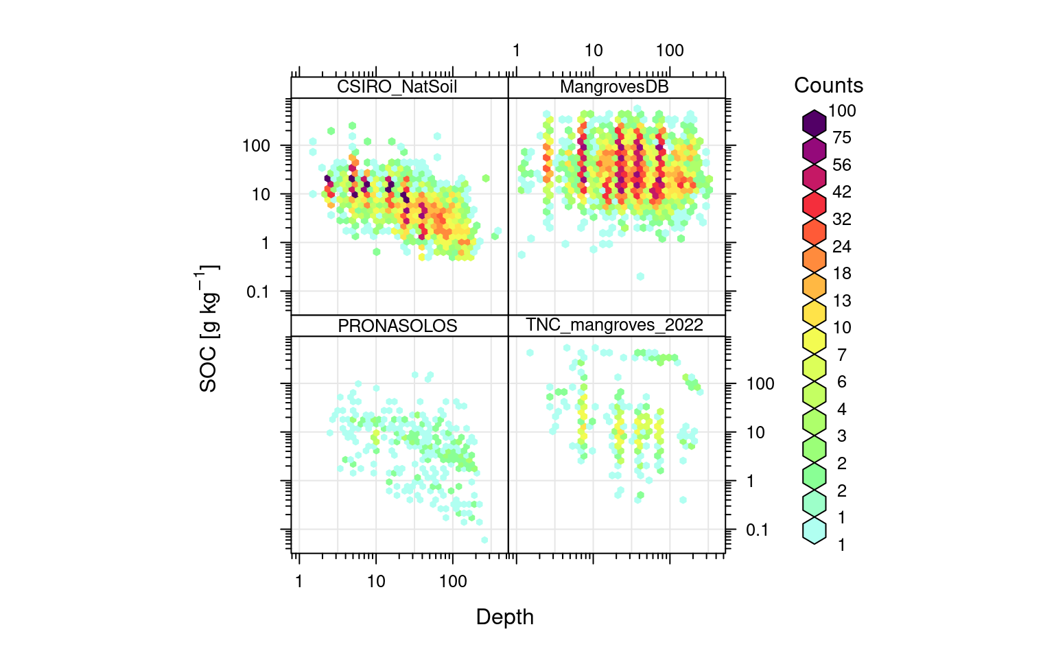

Distribution of values for SOC in g/kg vs soil depth. Notice for many soil samples standard depths are used hence some groupings are visible.

Figure 6.3: Distribution of values for SOC in g/kg vs soil depth. Notice for many soil samples standard depths are used hence some groupings are visible.

In this case clearly most of soils in mangrove forests are so-called organic soils where SOC content remains high with depth (compare vs CSIRO samples from Australia and PRONASOLOS samples from Brazil). We can quickly estimate what the average SOC content for world mangroves by using:

sel.oc = rms.df$source_db %in% c("MangrovesDB","TNC_mangroves_2022")
mean.oc = mean(rms.df[sel.oc,"oc"], na.rm=TRUE)
mean.oc
#> [1] 56.50853
mean.hzn_depth = mean(rms.df[sel.oc,"hzn_depth"], na.rm=TRUE)
mean.hzn_depth
#> [1] 48.1298

Hence world soil mangrove forest have about 5.6% SOC for an average soil depth of 48-cm. Next we can look at the bulk density values:

openair::scatterPlot(rms.df[sel.db,], y = "db_od", x = "oc", method = "hexbin", col = "increment", type = "source_db", log.x = TRUE, ylab="BD", xlab="SOC [g/kg]")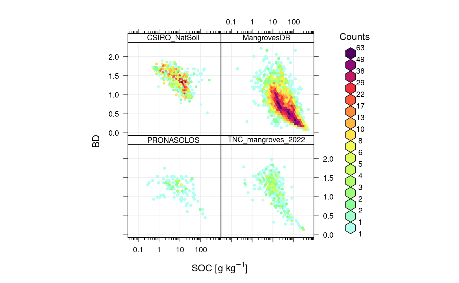

Figure 6.4: Distribution of values for SOC in g/kg vs soil bulk density.

This shows that, as expected BD can be related with SOC using linear-log relationship. Note that most of bulk density points in Sanderman et al. (2018) (MangrovesDB) are based on using a simple pedo-transfer function to estimate BD from SOC content. In reality there are usually much less soil laboratory samples available with actual BD measured in the lab. We can use actual SOC and BD measurements to estimate a more applicable pedo-transfer function for bulk density:

m.bd.soc = lm(db_od~log1p(oc)+log1p(hzn_depth), rms.df[!rms.df$source_db %in% c("MangrovesDB"),])
summary(m.bd.soc)
#> 
#> Call:
#> lm(formula = db_od ~ log1p(oc) + log1p(hzn_depth), data = rms.df[!rms.df$source_db %in% 
#>     c("MangrovesDB"), ])
#> 
#> Residuals:
#>      Min       1Q   Median       3Q      Max 
#> -1.17797 -0.14048  0.01392  0.14586  1.20172 
#> 
#> Coefficients:
#>                   Estimate Std. Error t value Pr(>|t|)    
#> (Intercept)       2.212642   0.018520  119.47   <2e-16 ***
#> log1p(oc)        -0.293363   0.003475  -84.43   <2e-16 ***
#> log1p(hzn_depth) -0.065487   0.004382  -14.95   <2e-16 ***
#> ---
#> Signif. codes:  0 '***' 0.001 '**' 0.01 '*' 0.05 '.' 0.1 ' ' 1
#> 
#> Residual standard error: 0.2323 on 2885 degrees of freedom
#>   (3914 observations deleted due to missingness)
#> Multiple R-squared:  0.7142, Adjusted R-squared:  0.714 
#> F-statistic:  3604 on 2 and 2885 DF,  p-value: < 2.2e-16

so that we can estimate bulk density for average SOC content and depth of 50-cm:

mean.db_od = predict(m.bd.soc, data.frame(oc=mean.oc, hzn_depth=mean.hzn_depth))
mean.db_od
#>         1 
#> 0.7689179

i.e. it is about 770 kg/m-cubic. Based on these rough numbers we can estimate that the mean SOC density for world mangroves at 50-cm depth is about:

mean.oc/1000 * mean.db_od * 1000
#>        1 
#> 43.45042

i.e. about 43 kg/m-cubic, so that the total SOC stock for 0–100 cm is about 430 t/ha. Assuming that there are about 147,000 square-km of mangroves forests in the world, this would estimate total SOC stock for 0–100 cm to be:

430 * 147e3 * 100 / 1e9
#> [1] 6.321

i.e. about 6.3 gigatones of soil carbon. This estimate is not ideal for multiple reasons:

Training points are just a compilation of data from literature, i.e. it is possible that some areas are over-represented i.e. that there is a bias in how average SOC is estimated,
Training points come from different time-periods and SOC is a dynamic property; again we could generate bias in predictions,

6.4 Pedo-tranfer function to estimate SOC density from content

We can also look at relationship between SOC (%) and SOC density (kg/m3). Based on the available data this shows:

openair::scatterPlot(rms.df[sel.db,], y = "oc_d", x = "oc", method = "hexbin", col = "increment", type = "source_db", log.x = TRUE, log.y = TRUE, ylab="SOC [kg/m3]", xlab="SOC [g/kg]")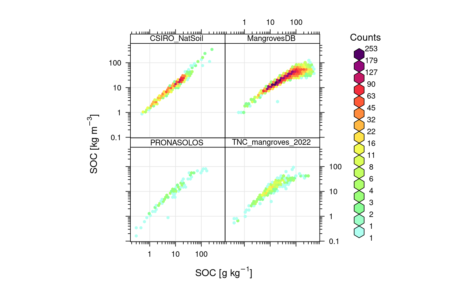

Figure 6.5: Relationship between SOC content and density on a log-scale.

Which shows that SOC in kg/m3 is log-linearly correlated with SOC %, except for organic soils this relationship is curvilinear i.e. after some values of SOC % SOC in kg/m3 stabilizes and does not grow any more. Again, we can fit a simple pedo-transfer function using this data to predict SOC density (kg/m3) directly from SOC %:

rms.df$log.oc2 = rms.df$log.oc^2
df.oc_d = rms.df[sel.oc,c("oc_d", "log.oc", "log.oc2", "hzn_depth")]
## remove some artifacts in points:
df.oc_d = df.oc_d[!(df.oc_d$log.oc<0.5 & df.oc_d$oc_d>5),]
m.oc_d = glm(I(oc_d+.Machine$double.eps)~log.oc+log.oc2+hzn_depth, 
             df.oc_d, family = gaussian(link="log"))
summary(m.oc_d)
#> 
#> Call:
#> glm(formula = I(oc_d + .Machine$double.eps) ~ log.oc + log.oc2 + 
#>     hzn_depth, family = gaussian(link = "log"), data = df.oc_d)
#> 
#> Deviance Residuals: 
#>     Min       1Q   Median       3Q      Max  
#> -28.255   -2.370    0.317    1.724   71.752  
#> 
#> Coefficients:
#>               Estimate Std. Error t value Pr(>|t|)    
#> (Intercept) -8.345e-01  6.701e-02 -12.455  < 2e-16 ***
#> log.oc       1.651e+00  3.170e-02  52.094  < 2e-16 ***
#> log.oc2     -1.404e-01  3.687e-03 -38.085  < 2e-16 ***
#> hzn_depth    3.423e-04  6.555e-05   5.222 1.84e-07 ***
#> ---
#> Signif. codes:  0 '***' 0.001 '**' 0.01 '*' 0.05 '.' 0.1 ' ' 1
#> 
#> (Dispersion parameter for gaussian family taken to be 49.05412)
#> 
#>     Null deviance: 1511634  on 5564  degrees of freedom
#> Residual deviance:  272790  on 5561  degrees of freedom
#>   (52 observations deleted due to missingness)
#> AIC: 37463
#> 
#> Number of Fisher Scoring iterations: 5

This models has an R-square of about:

#calculate McFadden's R-squared for model
with(summary(m.oc_d), 1 - deviance/null.deviance)
#> [1] 0.8195399

We can plot the fitted model vs measured data by using:

oc_data <- data.frame(log.oc=seq(0, 6, length.out=20))
oc_data$log.oc2 = oc_data$log.oc^2
oc_data$hzn_depth = 20
oc_data$oc_d = predict(m.oc_d, oc_data, type = c("response"))
ggplot(df.oc_d, aes(log.oc, oc_d)) + 
  geom_hex(bins=40) + 
  scale_fill_gradient(low = "grey90", high = "black") +
  theme_bw() + 
  geom_line(data=oc_data, aes(log.oc, oc_d), col="orange",
              size=1)
#> Warning: Removed 52 rows containing non-finite values (stat_binhex).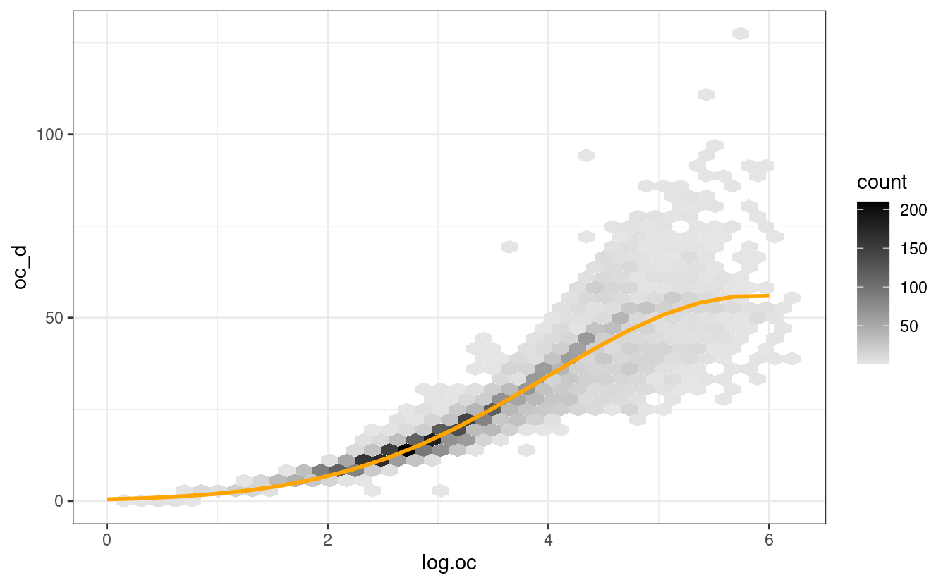

Modelling SOC density (kg/m3) as a function of log.SOC (g/kg). This model explains cca 80% of variability in data, notice however that the uncertainty around regression line increases for higher values of SOC.

Figure 6.6: Modelling SOC density (kg/m3) as a function of log.SOC (g/kg). This model explains cca 80% of variability in data, notice however that the uncertainty around regression line increases for higher values of SOC.

This means that at depth of 20-cm, SOC % of 6% (log.SOC = 4.1) converts to SOC density (kg/m3) of about 36 kg/m-cubic, but the number could very well be somewhere between 22 and 46 kg/m-cubic (see density plot above).

oc_data$SOC = expm1(oc_data$log.oc)
oc_data[14,c("SOC","log.oc","oc_d")]
#>         SOC   log.oc     oc_d
#> 14 59.65871 4.105263 36.03792

6.5 Estimating total stocks using Predictive Soil Mapping

In the previous examples we have shown how to start with checking the SOC data to estimate global stocks, visualize relationships and detect differences between datasets. The quick-and-dirt calculus tells us that there should be about 6.3 gigatones of soil carbon in the world mangrove forests. This number assumes perfectly random sample and no bias in representation of various geographies and soil depths.

To produce a more reliable estimate of global SOC stock in world mangroves and also to map their distribution we will use predictive soil mapping, in this case spatiotemporal Ensemble Machine Learning (EML) and the approach where SOC (g/kg) and BD are used independently, then aggregated to derive SOC stocks.

We can first check if there is enough point data spread through time:

openair::scatterPlot(rms.df[sel.db,], y = "oc", x = "observation_year", method = "hexbin", type = "source_db", col = "increment", log.y = TRUE, xlab="Year", ylab="SOC [g/kg]")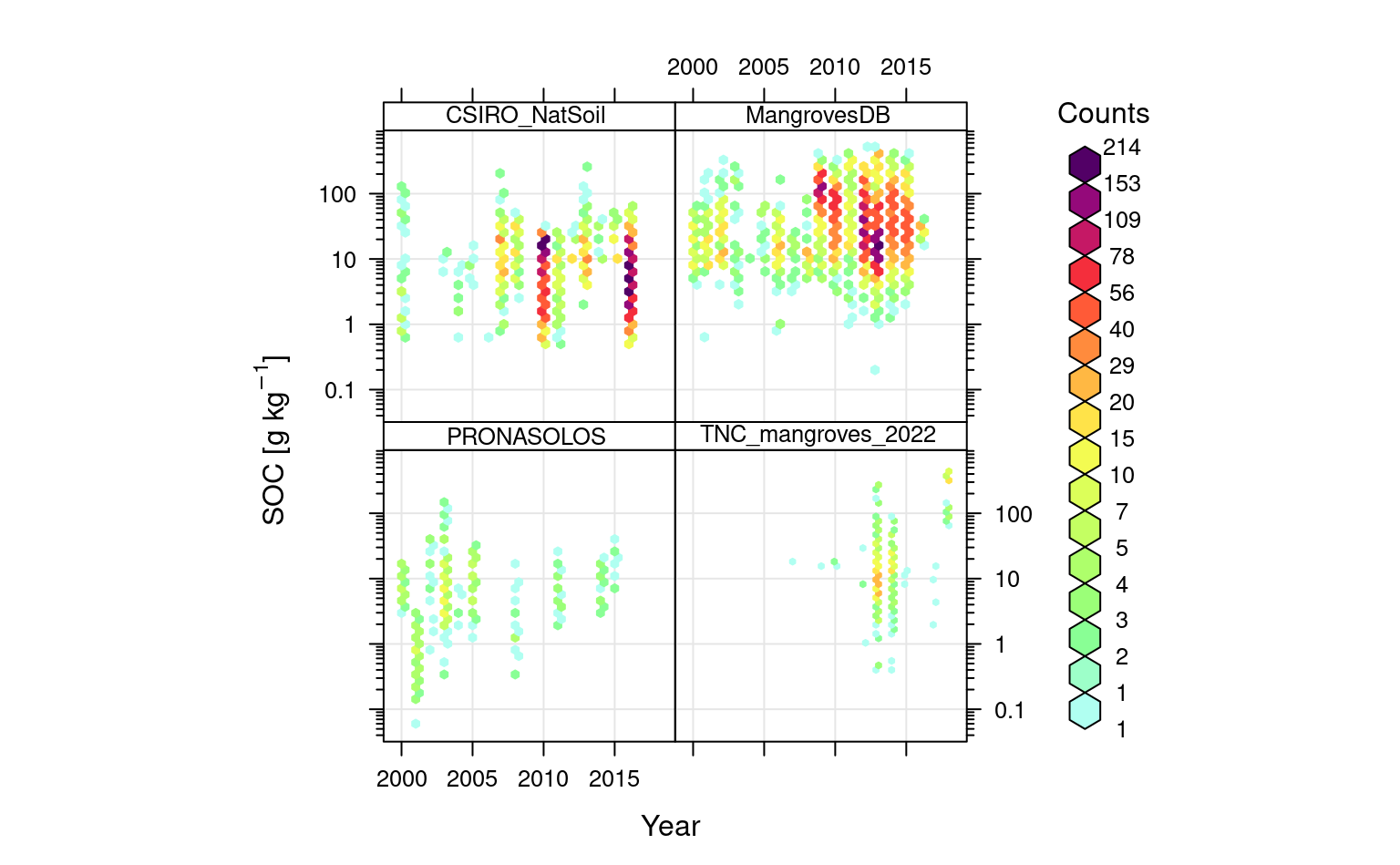

Figure 6.7: Distribution of training points through time.

Overall, there are definitively enough points spread over time for spatiotemporal mapping of SOC. Also note, there seems to be, in average, no overall trends in SOC. Still, many reports shows that in some areas such as Niger delta, Indonesia, Australia etc the mangrove forests have gone through significant degradation (Leal & Spalding, 2022; Murray et al., 2022) and this should be also represented in maps.

6.6 Estimating added value of temporal component

For spatiotemporal EML we use a regression matrix with number of target variables, and over 150 covariate layers. This include:

Globally consistent time-series 2000–2020 ARD Landsat bands (Blue, Green, Red, NIR, SWIR1, SWIR2) (Potapov et al., 2020), aggregated and gap-filled to produce complete consistent lower quantiles (P25 = lower 0.25 probability), as explained in detail in Yamazaki et al. (2019),
Time-series of CHELSA images representing climate precipitation, mean, minimum and maximum air temperature (Karger et al., 2017),
MODIS LST (1km) and EVI (250m) monthly time-series (covering 2000–2020 period) generated using aggregation,
Number of static (long-term) layers including MERIT DEM elevation (Yamazaki et al., 2019), global surface water probability (Pekel, Cottam, Gorelick, & Belward, 2016), long-term climatic variables and and global composites of Landsat bands from 2010, 2014 and 2018 (Hansen et al., 2013),

In addition to original Landsat bands, we also use a list of standard vegetation indices that can be derived from Landsat data. The Landsat bands and derivatives are available at 30-m spatial resolution, while the 250m and 1km resolution images had to be downscaled to 30-m spatial resolution (here we used GDAL and cubic-spline downscaling). An example of complete data prepared for world mangroves is the tile 162E_10S:

g30m.t = readRDS("./input/T162E_10S/data_2020.rds")
dim(g30m.t@data)
#> [1] 10548   147
g30m.s = readRDS("./input/T162E_10S/data_static.rds")
str(g30m.s@data)
#> 'data.frame':    10548 obs. of  18 variables:
#>  $ band1                               : int  1 1 1 1 1 1 1 1 1 1 ...
#>  $ Landsat_treecover2000               : num  6 4 8 5 12 7 5 3 2 1 ...
#>  $ Landsat2000_NIR                     : num  62 57 66 65 68 68 67 64 59 52 ...
#>  $ Landsat2000_red                     : num  39 37 40 39 39 40 39 38 35 32 ...
#>  $ Landsat2000_SWIR1                   : num  41 41 49 51 50 52 53 53 50 44 ...
#>  $ Landsat2000_SWIR2                   : num  10 10 14 15 16 18 19 18 17 15 ...
#>  $ Landsat2014_NIR                     : num  59 51 60 60 63 63 62 58 51 42 ...
#>  $ Landsat2014_red                     : num  36 36 32 33 27 30 32 32 32 29 ...
#>  $ Landsat2014_SWIR1                   : num  40 38 43 47 42 46 49 48 42 34 ...
#>  $ Landsat2014_SWIR2                   : num  11 10 13 15 15 17 19 18 16 12 ...
#>  $ Landsat2018_NIR                     : num  43 32 37 34 45 43 42 40 36 32 ...
#>  $ Landsat2018_red                     : num  38 36 38 38 39 40 40 41 41 40 ...
#>  $ Landsat2018_SWIR1                   : num  34 29 33 32 37 37 37 36 34 31 ...
#>  $ Landsat2018_SWIR2                   : num  16 14 16 16 18 18 18 18 17 15 ...
#>  $ MERIT_height.above.nearest.neighbour: num  0.00 0.00 3.69e-07 0.00 1.01e-04 ...
#>  $ MERIT_upstream.area                 : num  0.2445 0.2303 0.0768 0.0971 0.0389 ...
#>  $ Water_change                        : num  242 238 248 247 251 250 247 241 231 217 ...
#>  $ Water_occurrence                    : num  35 41 27 29 19 21 24 30 39 49 ...

We can start modeling SOC by testing predictive power of purely-spatial vs spatiotemporal covariates. We first test modeling performance using only static covariates and log-SOC (%) as the target variable:

pr.vars = readRDS("./input/world.mangroves_soil.carbon_pr.vars.rds")
pr.vars0 = names(g30m.s@data)[-1]
sel0 = complete.cases(rms.df[,c("log.oc", pr.vars0)])
m0.oc = ranger::ranger(y=rms.df$log.oc[sel0], x=rms.df[sel0, c("hzn_depth", pr.vars0)], 
            num.trees = 85, importance = 'impurity')
m0.oc
#> Ranger result
#> 
#> Call:
#>  ranger::ranger(y = rms.df$log.oc[sel0], x = rms.df[sel0, c("hzn_depth",      pr.vars0)], num.trees = 85, importance = "impurity") 
#> 
#> Type:                             Regression 
#> Number of trees:                  85 
#> Sample size:                      11903 
#> Number of independent variables:  18 
#> Mtry:                             4 
#> Target node size:                 5 
#> Variable importance mode:         impurity 
#> Splitrule:                        variance 
#> OOB prediction error (MSE):       0.3291843 
#> R squared (OOB):                  0.8198406

sel1 = complete.cases(rms.df[,c("log.oc", pr.vars)])
m1.oc = ranger::ranger(y=rms.df$log.oc[sel1], x=rms.df[sel1, c("hzn_depth", pr.vars)], 
            num.trees = 85, importance = 'impurity')
m1.oc
#> Ranger result
#> 
#> Call:
#>  ranger::ranger(y = rms.df$log.oc[sel1], x = rms.df[sel1, c("hzn_depth",      pr.vars)], num.trees = 85, importance = "impurity") 
#> 
#> Type:                             Regression 
#> Number of trees:                  85 
#> Sample size:                      9275 
#> Number of independent variables:  156 
#> Mtry:                             12 
#> Target node size:                 5 
#> Variable importance mode:         impurity 
#> Splitrule:                        variance 
#> OOB prediction error (MSE):       0.3305873 
#> R squared (OOB):                  0.8076966

It appears that static variables are already sufficient to map SOC content and the models are highly significant. The problem of this approach is that it ignores spatial clustering of points including the fact that many samples come from the same spatial locations. We want to, instead, validate models using spatial blocks so that a subset of points is either used for training or cross-validation. To fit a model that blocks spatially overlapping points into training or validation we can use the mlr package:

lrns <- list(mlr::makeLearner("regr.ranger", 
                num.threads = parallel::detectCores(), num.trees=85, importance="impurity"),
             mlr::makeLearner("regr.cubist"), mlr::makeLearner("regr.rpart"), 
             mlr::makeLearner("regr.cvglmnet"))
tsk0 <- mlr::makeRegrTask(data = rms.df[sel0, c("log.oc", "hzn_depth", pr.vars0)], 
                          blocking = as.factor(rms.df$ID[sel0]), 
                          target = "log.oc")
init.m <- mlr::makeStackedLearner(lrns, method = "stack.cv", 
                                  super.learner = "regr.lm",
                                  resampling=mlr::makeResampleDesc(method = "CV", blocking.cv=TRUE))
eml0 = train(init.m, tsk0)
#> Exporting objects to slaves for mode socket: .mlr.slave.options
#> Mapping in parallel: mode = socket; level = mlr.resample; cpus = 32; elements = 10.
#> Exporting objects to slaves for mode socket: .mlr.slave.options
#> Mapping in parallel: mode = socket; level = mlr.resample; cpus = 32; elements = 10.
#> Exporting objects to slaves for mode socket: .mlr.slave.options
#> Mapping in parallel: mode = socket; level = mlr.resample; cpus = 32; elements = 10.
#> Exporting objects to slaves for mode socket: .mlr.slave.options
#> Mapping in parallel: mode = socket; level = mlr.resample; cpus = 32; elements = 10.
summary(eml0$learner.model$super.model$learner.model)
#> 
#> Call:
#> stats::lm(formula = f, data = d)
#> 
#> Residuals:
#>     Min      1Q  Median      3Q     Max 
#> -4.2041 -0.6227 -0.0291  0.5827  4.3693 
#> 
#> Coefficients:
#>               Estimate Std. Error t value Pr(>|t|)    
#> (Intercept)    0.02591    0.03257   0.795    0.426    
#> regr.ranger    0.58974    0.02487  23.712   <2e-16 ***
#> regr.cubist    0.09110    0.00806  11.302   <2e-16 ***
#> regr.rpart     0.02610    0.01996   1.308    0.191    
#> regr.cvglmnet  0.27673    0.02389  11.581   <2e-16 ***
#> ---
#> Signif. codes:  0 '***' 0.001 '**' 0.01 '*' 0.05 '.' 0.1 ' ' 1
#> 
#> Residual standard error: 0.9917 on 11898 degrees of freedom
#> Multiple R-squared:  0.462,  Adjusted R-squared:  0.4618 
#> F-statistic:  2554 on 4 and 11898 DF,  p-value: < 2.2e-16

In this case we have added ID which is the unique ID of the spatial block (30×30-km). So the results show drastically lower R-square when strict spatial blocking is used: e.g. a drop from 0.82 to 0.44. The drop in R-square is primarily effect of taking complete soil profiles and points close to each other out of training (Gasch et al., 2015).

We can compare accuracy of modeling with using both statics and temporal variables:

tsk1 <- mlr::makeRegrTask(data = rms.df[sel1, c("log.oc", "hzn_depth", pr.vars)], 
                          blocking = as.factor(rms.df$ID[sel1]), 
                          target = "log.oc")
eml1 = train(init.m, tsk1)
#> Exporting objects to slaves for mode socket: .mlr.slave.options
#> Mapping in parallel: mode = socket; level = mlr.resample; cpus = 32; elements = 10.
#> Exporting objects to slaves for mode socket: .mlr.slave.options
#> Mapping in parallel: mode = socket; level = mlr.resample; cpus = 32; elements = 10.
#> Exporting objects to slaves for mode socket: .mlr.slave.options
#> Mapping in parallel: mode = socket; level = mlr.resample; cpus = 32; elements = 10.
#> Exporting objects to slaves for mode socket: .mlr.slave.options
#> Mapping in parallel: mode = socket; level = mlr.resample; cpus = 32; elements = 10.
summary(eml1$learner.model$super.model$learner.model)
#> 
#> Call:
#> stats::lm(formula = f, data = d)
#> 
#> Residuals:
#>     Min      1Q  Median      3Q     Max 
#> -3.8300 -0.5850 -0.0280  0.5595  3.5414 
#> 
#> Coefficients:
#>                Estimate Std. Error t value Pr(>|t|)    
#> (Intercept)    0.099573   0.028541   3.489 0.000488 ***
#> regr.ranger    0.786823   0.021184  37.143  < 2e-16 ***
#> regr.cubist    0.064157   0.005681  11.293  < 2e-16 ***
#> regr.rpart     0.141459   0.016134   8.768  < 2e-16 ***
#> regr.cvglmnet -0.030274   0.012225  -2.476 0.013290 *  
#> ---
#> Signif. codes:  0 '***' 0.001 '**' 0.01 '*' 0.05 '.' 0.1 ' ' 1
#> 
#> Residual standard error: 0.9216 on 9270 degrees of freedom
#> Multiple R-squared:  0.5062, Adjusted R-squared:  0.506 
#> F-statistic:  2375 on 4 and 9270 DF,  p-value: < 2.2e-16

This shows that: (1) adding temporal components helps increase mapping accuracy although the difference is marginal (e.g. 5–10%), (2) without using CV with blocking, Random Foreost most likely overfits training points.

The estimated accuracy of predicting SOC content (%) anywhere in the world (inside the world mangrove forests) is thus:

t.b = quantile(rms.df$log.oc, c(0.001, 0.01, 0.999), na.rm=TRUE)
plot_hexbin(varn="SOC_EML", breaks=c(t.b[1], seq(t.b[2], t.b[3], length=25)), 
      meas=eml1$learner.model$super.model$learner.model$model$log.oc, 
      pred=eml1$learner.model$super.model$learner.model$fitted.values, 
      main="SOC [EML]")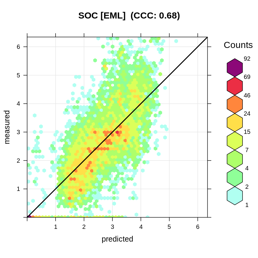

Figure 6.8: Accuracy plot for soil organic carbon fitted using Ensemble ML.

It is also interesting to look at the variable importance for this model to see which covariates are most important for modeling SOC:

library(ggplot2)
xl.soc <- as.data.frame(mlr::getFeatureImportance(eml1[["learner.model"]][["base.models"]][[1]])$res)
xl.soc$relative_importance = 100*xl.soc$importance/sum(xl.soc$importance)
xl.soc = xl.soc[order(xl.soc$relative_importance, decreasing = T),]
xl.soc$variable = paste0(c(1:nrow(xl.soc)), ". ", xl.soc$variable)
ggplot(data = xl.soc[1:20,], aes(x = reorder(variable, relative_importance), y = relative_importance)) +
  geom_bar(fill = "steelblue",
           stat = "identity") +
  coord_flip() +
  labs(title = "Variable importance",
       x = NULL,
       y = NULL) +
  theme_bw() + theme(text = element_text(size=15))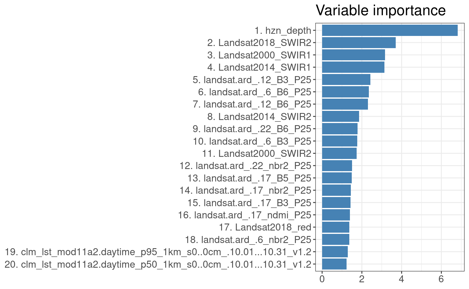

Figure 6.9: Variable importance for 3D prediction model for SOC based on random forest.

As expected, soil depth significantly helps predict SOC. Next most important covariates are Landsat SWIR bands and daytime surface temperature (LST) for October. Note that, in average, time-series landsat.ard (i.e. temporal component) are overall the most important covariates.

Likewise, we can fit an independent model for BD using the same modeling framework:

sel.bd = complete.cases(rms.df[,c("db_od", pr.vars)])
tsk.bd <- mlr::makeRegrTask(data = rms.df[sel.bd, c("db_od", "hzn_depth", pr.vars)], 
                          blocking = as.factor(rms.df$ID[sel.bd]), 
                          target = "db_od")
bd.eml = train(init.m, tsk.bd)
#> Exporting objects to slaves for mode socket: .mlr.slave.options
#> Mapping in parallel: mode = socket; level = mlr.resample; cpus = 32; elements = 10.
#> Exporting objects to slaves for mode socket: .mlr.slave.options
#> Mapping in parallel: mode = socket; level = mlr.resample; cpus = 32; elements = 10.
#> Exporting objects to slaves for mode socket: .mlr.slave.options
#> Mapping in parallel: mode = socket; level = mlr.resample; cpus = 32; elements = 10.
#> Exporting objects to slaves for mode socket: .mlr.slave.options
#> Mapping in parallel: mode = socket; level = mlr.resample; cpus = 32; elements = 10.
summary(bd.eml$learner.model$super.model$learner.model)
#> 
#> Call:
#> stats::lm(formula = f, data = d)
#> 
#> Residuals:
#>      Min       1Q   Median       3Q      Max 
#> -1.05477 -0.19936  0.00039  0.20085  1.37838 
#> 
#> Coefficients:
#>                Estimate Std. Error t value Pr(>|t|)    
#> (Intercept)    0.038527   0.013425   2.870  0.00412 ** 
#> regr.ranger    1.047436   0.019730  53.088  < 2e-16 ***
#> regr.cubist    0.039359   0.006733   5.846 5.35e-09 ***
#> regr.rpart    -0.107278   0.014905  -7.197 6.99e-13 ***
#> regr.cvglmnet  0.052440   0.018027   2.909  0.00364 ** 
#> ---
#> Signif. codes:  0 '***' 0.001 '**' 0.01 '*' 0.05 '.' 0.1 ' ' 1
#> 
#> Residual standard error: 0.3044 on 5328 degrees of freedom
#> Multiple R-squared:  0.5426, Adjusted R-squared:  0.5422 
#> F-statistic:  1580 on 4 and 5328 DF,  p-value: < 2.2e-16

This has more missing values and is hence will likely be more cumbersome to map at higher accuracy. Note that the residual error (RMSE) of 294 kg/m3 is relatively high, which means that with our model we can only detect about 11 classes of BD (Tomislav Hengl, Nikolić, & MacMillan, 2013):

bd.range = quantile(rms.df$db_od, probs=c(0.01, 0.99), na.rm=TRUE)
round(diff(bd.range)/(0.293/2))
#> 99% 
#>  11

The classes would be e.g.:

seq(bd.range[1], bd.range[2], length.out=round(diff(bd.range)/(0.293/2)))
#>  [1] 0.1332139 0.2998925 0.4665711 0.6332497 0.7999283 0.9666069 1.1332855
#>  [8] 1.2999642 1.4666428 1.6333214 1.8000000

6.7 Producing predictions of SOC and BD

Now that we have fitted (independently) models for SOC and BD, we can generate predictions for all time-periods and all standard depths (0, 30, 60 and 100-cm). Then, after we produce predictions at standard depths, we can aggregate those predictions to standard depth intervals e.g. 0–30 and 30–100 cm. For each interval, we can then determine SOC stocks (t/ha) and then sum up the two to produce total SOC stocks 0–100 cm.

In summary, we will produce a total of 190+ maps, which includes:

Predictions of SOC and BD at 4 standard depths + prediction errors for 5 period (2×4×2×5 = 96),
Derived values for SOC and BD for standard depth intervals 0–30 and 30–100-cm (2×2×2×5 = 40),
Derived stocks for standard depths with lower and upper intervals (2×3×5 = 30),

The 4-year time-periods include:

2002 = 2000–2003,
2006 = 2004–2007,
2010 = 2008–2011,
2014 = 2012–2015,
2018 = 2016–2019,
2020 = 2020–2021,

We first prepare a function pred_mlr and pred_lst (see R script PSM_functions.R) to speed up making predictions. We can now run predictions over time-periods:

source("PSM_functions.R")
yl =  c(2002, 2006, 2010, 2014, 2018, 2020)
## correction factor for prediction error:
m.train = eml1$learner.model$super.model$learner.model$model
m.terms = all.vars(eml1$learner.model$super.model$learner.model$terms)
eml.MSE0 = matrixStats::rowSds(as.matrix(m.train[,m.terms[-1]]), na.rm=TRUE)^2
eml.MSE = deviance(eml1$learner.model$super.model$learner.model)/df.residual(eml1$learner.model$super.model$learner.model)
## correction factor:
eml.cf = eml.MSE/mean(eml.MSE0, na.rm = TRUE)
for(year in yl){
  try( pred_lst(tvar="log.oc", id="T162E_10S", year, eml1, eml.cf, in.dir="./input/") )
}

Next, we can aggregate all predictions to produce SOC and BD estimates for standard depth intervals. For this we use the function soc_calc and we run it in parallel to speed up processing:

params = expand.grid(t.var=c("log.oc", "db.od"), year=yl, tile="T162E_10S")
params = split(params, 1:nrow(params))
#str(params[[1]])
library(doMC)
registerDoMC(parallel::detectCores())
x <- foreach(p=params, .packages=c("rgdal", "raster", "matrixStats"), 
             .export=c("agg_layers")) %dopar% 
     { agg_layers(year=p$year, t.var=p$t.var, tile=p$tile) }
## aggregate per tile
par0 = expand.grid(year=yl, tile="T162E_10S")
par0 = split(par0, 1:nrow(par0))
x <- foreach(p=par0, .packages=c("rgdal", "raster", "matrixStats"), .export=c("soc_calc", "OCSKGM")) %dopar%{ soc_calc(year=p$year, tile=p$tile) }

This will populate the folder ./output/T162E_10S with all maps as a result of predictive mapping. The most interesting output maps are e.g. sol_soc.tha_mangroves.typology_m_30m_s0..30cm_2020, which are the most recent estimates of SOC stocks for mangrove map of interest.

We can visualize produced predictions, best by using e.g. the Raster Time-series Manager plugin in QGIS or similar. Simply download the maps from the ./output/T162E_10S folder and open and customize predictions in QGIS as shown below. As you move with the cursor around the map, you will see changes in SOC stocks over different time-periods.

Figure 6.10: Visualization of SOC t/ha predictions in QGIS.

parallelMap::parallelStop()
#> Stopped parallelization. All cleaned up.

6.8 Comparing previous versions of SOC maps for mangroves

The previous model for SOC for mangroves was based on a somewhat smaller dataset with some additional covariates such as sea-surface-temperature and tidal range (Sanderman et al., 2018). We can again check the performance of the model using the strict cross-validation with blocking, this time we use the profile ID:

rm.oc = readRDS("./input/world.mangroves_soil.carbon_rm0.rds")
rm.oc$log.oc = log1p(rm.oc$ORCDRC)
fm.oc <- as.formula(paste0("log.oc ~ DEPTH + SOCS_0_200cm_30m + TRC_30m +
               SW1_30m + SW2_30m + SRTMGL1_30m + RED_30m + NIR_30m +", 
              paste0("SST_",c(1:4),"_30m", collapse="+"), "+", 
              paste0("TSM_",c(1:4),"_30m", collapse="+"), "+", 
              paste0("MTYP_",c("Organogenic","Mineralogenic","Estuarine"), 
                     "_30m", collapse = "+"), "+ TidalRange_30m"))

We again train the EML model by:

selA = complete.cases(rm.oc[,all.vars(fm.oc)])
tskA <- mlr::makeRegrTask(data = rm.oc[selA, all.vars(fm.oc)], 
                          blocking = as.factor(rm.oc$SOURCEID[selA]), 
                          target = "log.oc")
emlA = train(init.m, tskA)
summary(emlA$learner.model$super.model$learner.model)
#> 
#> Call:
#> stats::lm(formula = f, data = d)
#> 
#> Residuals:
#>     Min      1Q  Median      3Q     Max 
#> -4.3704 -0.2956  0.0384  0.3687  2.7122 
#> 
#> Coefficients:
#>                Estimate Std. Error t value Pr(>|t|)    
#> (Intercept)   -0.419323   0.038768 -10.816  < 2e-16 ***
#> regr.ranger    0.870707   0.018685  46.599  < 2e-16 ***
#> regr.cubist    0.021880   0.007254   3.016  0.00257 ** 
#> regr.rpart     0.143778   0.019601   7.335 2.47e-13 ***
#> regr.cvglmnet  0.084548   0.021101   4.007 6.22e-05 ***
#> ---
#> Signif. codes:  0 '***' 0.001 '**' 0.01 '*' 0.05 '.' 0.1 ' ' 1
#> 
#> Residual standard error: 0.6792 on 6618 degrees of freedom
#> Multiple R-squared:  0.6747, Adjusted R-squared:  0.6745 
#> F-statistic:  3432 on 4 and 6618 DF,  p-value: < 2.2e-16

tskB <- mlr::makeRegrTask(data = rms.df[sel1, c("log.oc", "hzn_depth", pr.vars)], 
                          blocking = as.factor(rms.df$olc_id[sel1]), 
                          target = "log.oc")
emlB = train(init.m, tskB)
summary(emlB$learner.model$super.model$learner.model)
#> 
#> Call:
#> stats::lm(formula = f, data = d)
#> 
#> Residuals:
#>     Min      1Q  Median      3Q     Max 
#> -3.3770 -0.3835  0.0076  0.3603  3.6555 
#> 
#> Coefficients:
#>                Estimate Std. Error t value Pr(>|t|)    
#> (Intercept)   -0.169293   0.022562  -7.504 6.78e-14 ***
#> regr.ranger    1.070425   0.017933  59.691  < 2e-16 ***
#> regr.cubist    0.108671   0.006921  15.701  < 2e-16 ***
#> regr.rpart     0.043195   0.014668   2.945  0.00324 ** 
#> regr.cvglmnet -0.154658   0.015597  -9.916  < 2e-16 ***
#> ---
#> Signif. codes:  0 '***' 0.001 '**' 0.01 '*' 0.05 '.' 0.1 ' ' 1
#> 
#> Residual standard error: 0.7126 on 9270 degrees of freedom
#> Multiple R-squared:  0.7047, Adjusted R-squared:  0.7046 
#> F-statistic:  5531 on 4 and 9270 DF,  p-value: < 2.2e-16

The R-square is somewhat higher than if we use 30×30km spatial blocking (strict), and still higher for the new set of covariates. Note that by blocking using only location ID, we generate a somewhat smaller RMSE; the true accuracy of predictions for SOC % is most likely somewhere between R-square of 0.50 and 0.70.

plot_hexbin(varn="SOC_EML_ID", breaks=c(t.b[1], seq(t.b[2], t.b[3], length=25)), 
      meas=emlB$learner.model$super.model$learner.model$model$log.oc, 
      pred=emlB$learner.model$super.model$learner.model$fitted.values, 
      main="SOC [EML] by ID")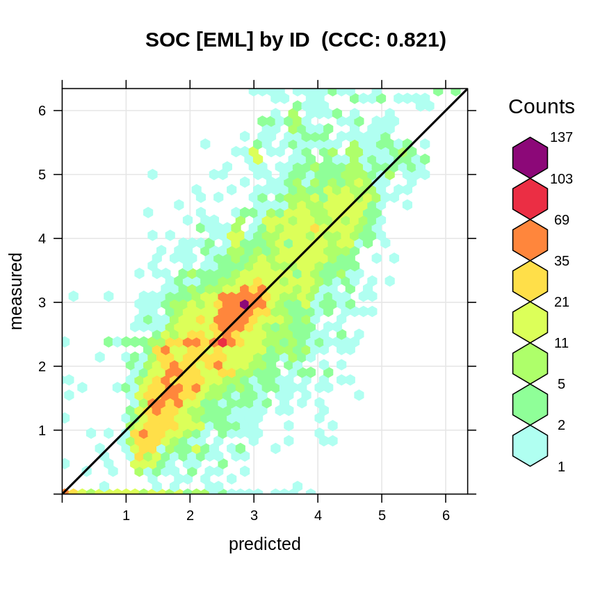

Figure 6.11: Accuracy plot for soil organic carbon fitted using Ensemble ML with blocking by profile ID only.

A comparison of predictions for an area shown below we notice that, by using the 30-m resolution covariate layers we produce much finer grain of detail, plus we most likely model SOC for deeper soils with higher accuracy / avoiding overfitting the models.

Figure 6.12: Comparing previous predictions of SOC at 100-m resolution vs current predictions at 30-m.

6.9 Removing uncertainty of predictions

As you can notice from the modeling results, uncertainty of predictions for SOC can be relatively large with R-square at CV points reaching max 0.5–0.7. To simplify decisions for decision-makers we can remove uncertainty from predictions by rounding all predictions using half-RMSE rule (Tomislav Hengl et al., 2013) i.e. by adjusting the numeric resolution of predictions.

Consider for example predictions of log-SOC % for 0–30 cm for the sample tile. We know that the average mapping accuracy (RMSE) for this variable is 0.914 (see previous sections), hence we can round all numbers using 0.914/2. This is an example:

library(terra)
#> terra 1.7.3
#> 
#> Attaching package: 'terra'
#> The following object is masked from 'package:landmap':
#> 
#>     makeTiles
#> The following object is masked from 'package:mlr':
#> 
#>     resample
#> The following object is masked from 'package:rgdal':
#> 
#>     project
oc.pred = terra::rast("./output/T162E_10S/sol_log.oc_mangroves.typology_m_30m_s0..30cm_2020_global_v0.1.tif")
names(oc.pred) = "log.oc"
oc.predB = as.data.frame(terra::crop(oc.pred, 
            ext(162.26889, 162.28905, -10.77543, -10.75329)), xy=TRUE)
oc.predB = oc.predB[!is.na(oc.predB$log.oc),]
oc.predB$CL = round(oc.predB$log.oc/10/(0.914/2))
oc.predB$s.log.oc = oc.predB$CL * 0.914/2 * 10
summary(as.factor(oc.predB$CL))
#>    7    8    9 
#>   41  396 1083

Assuming we want to know values with 67% probability confidence, then the map of SOC for this small area would only have 3 classes:

allN_df_long <- tidyr::pivot_longer(oc.predB, cols=c("log.oc","s.log.oc"))
lims = range(oc.predB$log.oc)
pal = RColorBrewer::brewer.pal(n=9, name = "RdYlGn")
ggplot() + 
  geom_raster(data = allN_df_long, aes(x=x, y=y, fill = value)) + 
  geom_path() + 
  facet_wrap(. ~ name, ncol = 2) + 
  scale_fill_gradientn(colours=pal, name="", limits=lims) + 
  theme_minimal() + xlab("Easting")+ ylab("Northing")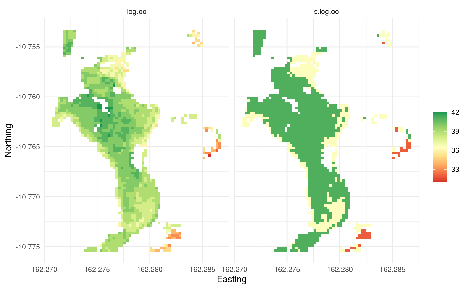

Figure 3.11: Predicted log-SOC original values (left) and rounded values using the average mapping accuracy.

Anyone wanting to use the maps for decisions without worrying about risks associated with uncertainty should probably use the map on the right. Likewise, uncertainty can also be used per pixel by combining the prediction errors with values and then deriving with 67% or 90% probability confidence areas exceeding some threshold value.

6.10 Summary points

In this tutorial we have demonstrated how to fit spatiotemporal models for SOC to estimate SOC stocks in t/ha (with prediction uncertainty) for the world mangrove forests. We fit two independent models for SOC content (%) and for bulk density, then aggregate values to produce global estimates of SOC for the whole mangroves. This is so-called 3D predictive soil mapping approach with independently fitted components of SOC stocks. For modeling we use a compilation of soil samples from literature and various national and international projects (at total of 12,000 samples). As covariate layers we use standard climatic, terrain, vegetation and hydrological parameters.

Results of strict cross-validation using 5-fold blocking (where spatially close points are used either for modeling or validation) show that the CCC for SOC (%) is about 0.7 and for bulk density (kg/m3) around 0.65. The mapping uncertainty is somewhat higher than for SOC mapping projects where interest is agricultural land. This is most likely due to the following reasons:

Most of world mangrove forests are in Tropics and covered with vegetation whole year; vegetation cover is not always linearly correlated with SOC content,
Point data (digitized from the literature mainly) used for training is largely unharmonized and many points have relatively inaccurate location,
A lot of SOC is located in deeper soils, so EO data only marginaly helps map SOC,

The tutorial demonstrates that Random Forest that ignores spatial overlap in training data would likely result in overfitting. This illustrates importance of doing strict validation to build models and interpret the results. As the most important covariates for mapping SOC models show soil depth and Landsat SWIR bands.

Based on spatiotemporal prediction of SOC stocks, we estimate that the global SOC stocks for world mangrove forests are in average about 350 t/ha for 0–100 cm depth (67% prob. interval: 232–470 t/ha) i.e. about 4.6 gigatonnes (67% prob. interval: 3.1–6.2), which is somewhat less than we estimate directly from soil samples. This is for 2 main probable reasons:

The soil samples (points) are usually collected for top-soil which usually has more SOC, hence average value from training points most likely over-estimates deeper soils,
Soil samples are in most cases collected inside mangrove forests, so that lower stocks in the transition areas would have also been likely over-estimated,

Also note that our results show that, in average, SOC for mangrove forests did not change (see below), although one would need to validate specifies areas to see if in some parts there are gains / losses in SOC. The figure below shows global mean and lower and upper prediction intervals for SOC stocks for mangrove forests through time.

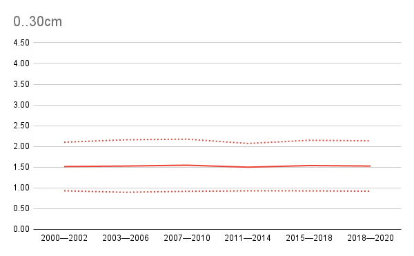
Figure 6.13: Global SOC stocks in gigatones with prediction uncertainty (+/- 1 std) for the time-period of interest.

6.11 Access global predictions of SOC for magroves

To access global predictions you can use the Cloud-Optimized GeoTIFFs available at https://s3.eu-central-1.wasabisys.com/openlandmap/mangroves/. Simply expand the file name using the file-name pattern of standard depths s0..30cm, s30..100cm and years of predictions e.g. 2020. Example of mean, lower-prediction-interval and upper-prediction-interval maps are:

soc.tha_tnc.mangroves.typology_m_30m_b0..100cm_2019_2020_go_epsg.4326_v1.2.tif,
soc.tha_tnc.mangroves.typology_l.std_30m_b0..100cm_2019_2020_go_epsg.4326_v1.2.tif,
soc.tha_tnc.mangroves.typology_u.std_30m_b0..100cm_2019_2020_go_epsg.4326_v1.2.tif,

From R you can access and crop this data using e.g.:

library(terra)
cog = "/vsicurl/https://s3.eu-central-1.wasabisys.com/openlandmap/mangroves/sol/soc.tha_tnc.mangroves.typology_m_30m_b0..100cm_2019_2020_go_epsg.4326_v1.2.tif"
terra::rast(cog)
#> class       : SpatRaster 
#> dimensions  : 288002, 1440002, 1  (nrow, ncol, nlyr)
#> resolution  : 0.00025, 0.00025  (x, y)
#> extent      : -180, 180.0005, -39.0005, 33  (xmin, xmax, ymin, ymax)
#> coord. ref. : lon/lat WGS 84 (EPSG:4326) 
#> source      : soc.tha_tnc.mangroves.typology_m_30m_b0..100cm_2019_2020_go_epsg.4326_v1.2.tif 
#> name        : soc.tha_tnc.mangroves.typology~cm_2019_2020_go_epsg.4326_v1.2

Once you define the COG in R, you can crop to bounding box of interest or simply overlay points or polygons.

Note: if you compare the output maps with the mask map of the global mangrove forests, you will notice that we could not produce predictions for about 116 mangroves polygons (mostly in Fiji and other smaller islands) because of the absence of GLAD Landsat data. We could try to predict these areas using only coarser resolution EO data, but the result would be highly uncertain + we would not match the spatial resolution, so we have decided to better leave the pixels as NA.

This work has received funding from the Global Mangrove Alliance. Global Mangrove Alliance is currently coordinated by members Conservation International, The International Union for the Conservation of Nature, The Nature Conservancy, Wetlands International and World Wildlife Fund.

5 Spatiotemporal Machine Learning for Species Distribution Modeling

7 Multi-scale spatial prediction models