4.1 Spatiotemporal interpolation of daily temperatures

In previous examples we have demonstrated effects of over-fitting and how Ensemble ML helps decrease overfitting and extrapolation problems using synthetic data. We can now look at some real-life cases for example the daily temperatures measured for several years for Croatia described in T. Hengl et al. (2012). This data sets consist of two parts: (1) measurements of daily temperatures at meteo stations, (2) list of gridded covariates (Fig. 4.1).

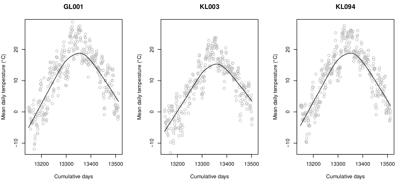
Figure 4.1: Temporal dynamics of mean-daily temperatures at sample meteorological stations. This shows seasonality effects (smoothed line) and daily oscillations.

We can load the point data by using:

library(rgdal)
hrmeteo = readRDS("input/hrtemp2006_meteo.rds")
str(hrmeteo)
#> List of 2
#>  $ meteo   :'data.frame':    44895 obs. of  5 variables:
#>   ..$ IDSTA : chr [1:44895] "GL001" "GL001" "GL001" "GL001" ...
#>   ..$ DATE  : chr [1:44895] "2006-1-1" "2006-1-2" "2006-1-3" "2006-1-4" ...
#>   ..$ MDTEMP: num [1:44895] 1.6 0.7 1.5 0.3 -0.1 1 0.3 -1.9 -5.4 -3.6 ...
#>   ..$ cday  : num [1:44895] 13148 13149 13150 13151 13152 ...
#>   .. ..- attr(*, "tzone")= chr ""
#>   ..$ x     : num [1:44895] NA NA NA NA NA NA NA NA NA NA ...
#>  $ stations:'data.frame':    152 obs. of  3 variables:
#>   ..$ IDSTA: chr [1:152] "GL001" "GL002" "GL003" "GL004" ...
#>   ..$ X    : num [1:152] 670760 643073 673778 752344 767729 ...
#>   ..$ Y    : num [1:152] 5083464 5086417 5052001 4726567 4717878 ...
idsta.pnts = hrmeteo$stations
coordinates(idsta.pnts) = ~ X + Y

This is a typical format for spatiotemporal meteorological data with locations of stations in one table, and measurements of daily temperatures (MDTEMP) in other. The column cday here is the cumulative day since 1970, which allows us to present time on a linear scale i.e. by using a numeric value instead of dates.

The gridded data includes: (a) static covariates (relief data), and (b) dynamic time-series data (MODIS LST). To load the static covariates we use:

hrgrid1km = readRDS("input/hrgrid1km.rds")
#plot(hrgrid1km[1])
proj4string(idsta.pnts) = proj4string(hrgrid1km)
str(hrgrid1km@data)
#> 'data.frame':    238630 obs. of  4 variables:
#>  $ HRdem : int  1599 1426 1440 1764 1917 1912 1707 1550 1518 1516 ...
#>  $ HRdsea: num  93 89.6 89.8 93.6 95 ...
#>  $ Lat   : num  46.5 46.5 46.5 46.5 46.5 ...
#>  $ Lon   : num  13.2 13.2 13.2 13.2 13.2 ...

The dynamic time-series data is stored in a local folder (input/LST2006HR) as individual files that we can list by using:

LST.listday <- dir("input/LST2006HR", pattern=glob2rx("LST2006_**_**.LST_Day_1km.tif"), full.names = TRUE)
LST.listnight <- dir("input/LST2006HR", pattern=glob2rx("LST2006_**_**.LST_Night_1km.tif"), full.names = TRUE)
str(LST.listday)
#>  chr [1:46] "input/LST2006HR/LST2006_01_01.LST_Day_1km.tif" ...

Here we see there are 46 images for year 2006 with daytime and 46 images for night time estimates of LST. We do not want to load all these rasters to R because we might experience RAM problems. We can first overlay points and see which variables can help with mapping daily temperatures.

For the static covariates we only have to run the overlay once:

idsta.ov <- sp::over(idsta.pnts, hrgrid1km)
idsta.ov$IDSTA = idsta.pnts$IDSTA
str(idsta.ov)
#> 'data.frame':    152 obs. of  5 variables:
#>  $ HRdem : int  161 134 202 31 205 563 80 96 116 228 ...
#>  $ HRdsea: num  198.5 181.7 192.9 0 1.5 ...
#>  $ Lat   : num  45.9 45.9 45.6 42.7 42.6 ...
#>  $ Lon   : num  17.2 16.8 17.2 18.1 18.3 ...
#>  $ IDSTA : chr  "GL001" "GL002" "GL003" "GL004" ...

For the spatiotemporal data (MODIS LST time-series) we need to run overlay as in a spacetime cube. This means that we need to match points using x,y,t coordinates with grids covering the same x,y,t fields. To speed up spacetime overlay we use our custom function extract_st, which basically builds on top of the terra package. First, we need to define begin, end times for each GeoTIFF:

library(terra)
source("mlst_functions.R")
hrmeteo$meteo$x = plyr::join(hrmeteo$meteo, hrmeteo$stations, by="IDSTA")$X
hrmeteo$meteo$y = plyr::join(hrmeteo$meteo, hrmeteo$stations, by="IDSTA")$Y
## generate row ID:
hrmeteo$meteo$row.id = 1:nrow(hrmeteo$meteo)
hrmeteo$meteo$Date = as.Date(hrmeteo$meteo$DATE, format = "%Y-%m-%d")
## strip dates from filename:
begin.tif1.lst = as.Date(paste0("2006-", substr(basename(LST.listday), 9, 10), 
                                "-", substr(basename(LST.listday), 12, 13)))-4
end.tif1.lst = as.Date(paste0("2006-", substr(basename(LST.listday), 9, 10), 
                              "-", substr(basename(LST.listday), 12, 13)))+4

now that we know spacetime coordinates for both points and grids, we can run overlay in parallel to speed up computing:

mc.cores = parallel::detectCores()
ov.pnts <- parallel::mclapply(1:length(LST.listday), function(i){ 
  extract_st(tif=LST.listday[i], hrmeteo$meteo, date="Date", 
             crs = proj4string(hrgrid1km),        
             date.tif.begin=begin.tif1.lst[i], 
             date.tif.end=end.tif1.lst[i], 
             coords=c("x","y"), variable.name="LST.day") }, 
  mc.cores=mc.cores)
ov.pnts = ov.pnts[!sapply(ov.pnts, is.null)]
ov.tifs1 = plyr::join_all(ov.pnts, by="row.id", type="full")
str(ov.tifs1)
#> 'data.frame':    44895 obs. of  2 variables:
#>  $ LST.day: int  0 0 0 0 0 0 0 0 0 0 ...
#>  $ row.id : int  1 2 3 4 5 366 367 368 369 370 ...
ov.tifs1$LST.day = ifelse(ov.tifs1$LST.day == 0, NA, ov.tifs1$LST.day)

In this case we also exclude the values of LST.day are equal to 0 as these are basically missing values in the GeoTIFFs. We repeat the same overlay operation for the night light images:

begin.tif2.lst = as.Date(paste0("2006-", substr(basename(LST.listnight), 9, 10), 
                                "-", substr(basename(LST.listnight), 12, 13)))-4
end.tif2.lst = as.Date(paste0("2006-", substr(basename(LST.listnight), 9, 10), 
                              "-", substr(basename(LST.listnight), 12, 13)))+4
ov.pnts <- parallel::mclapply(1:length(LST.listnight), function(i){ 
  extract_st(tif=LST.listnight[i], hrmeteo$meteo, date="Date", 
             crs = proj4string(hrgrid1km),        
             date.tif.begin=begin.tif2.lst[i], 
             date.tif.end=end.tif2.lst[i], 
             coords=c("x","y"), variable.name="LST.night") }, 
  mc.cores=mc.cores)
ov.pnts = ov.pnts[!sapply(ov.pnts, is.null)]
ov.tifs2 = plyr::join_all(ov.pnts, by="row.id", type="full")
str(ov.tifs2)
#> 'data.frame':    44895 obs. of  2 variables:
#>  $ LST.night: int  13344 13344 13344 13344 13344 13120 13120 13120 13120 13120 ...
#>  $ row.id   : int  1 2 3 4 5 366 367 368 369 370 ...
ov.tifs2$LST.night = ifelse(ov.tifs2$LST.night == 0, NA, ov.tifs2$LST.night)

The result of spacetime overlay is a simple long table matching exactly the meteo-data table. We next bind results of overlay using static and dynamic covariates:

hrmeteo.rm = plyr::join_all(list(hrmeteo$meteo, ov.tifs1, ov.tifs2))
#> Joining by: row.id
#> Joining by: row.id
hrmeteo.rm = plyr::join(hrmeteo.rm, idsta.ov)
#> Joining by: IDSTA

we also add the geometric component of temperature based on the sphere formulas:

hrmeteo.rm$temp.mean <- temp.from.geom(fi=hrmeteo.rm$Lat, 
                   as.numeric(strftime(hrmeteo.rm$Date, format = "%j")), 
                   a=37.03043, b=-15.43029, elev=hrmeteo.rm$HRdem, t.grad=0.6)

We have now produced a spatiotemporal regression matrix that can be used to fit a prediction model for daily temperature. The model is of form:

fm.tmp <- MDTEMP ~ temp.mean + LST.day + LST.night + HRdsea

We next fit an Ensemble ML using the same process described in the previous sections:

library(mlr)
lrn.rf = mlr::makeLearner("regr.ranger", num.trees=150, importance="impurity",
                          num.threads = parallel::detectCores())
lrns.st <- list(lrn.rf, mlr::makeLearner("regr.nnet"), mlr::makeLearner("regr.gamboost"))
sel = complete.cases(hrmeteo.rm[,all.vars(fm.tmp)])
hrmeteo.rm = hrmeteo.rm[sel,]
#summary(sel)
subs <- runif(nrow(hrmeteo.rm))<.2
tsk0.st <- mlr::makeRegrTask(data = hrmeteo.rm[subs,all.vars(fm.tmp)], 
                             target = "MDTEMP", blocking = as.factor(hrmeteo.rm$IDSTA[subs]))
tsk0.st
#> Supervised task: hrmeteo.rm[subs, all.vars(fm.tmp)]
#> Type: regr
#> Target: MDTEMP
#> Observations: 7573
#> Features:
#>    numerics     factors     ordered functionals 
#>           4           0           0           0 
#> Missings: FALSE
#> Has weights: FALSE
#> Has blocking: TRUE
#> Has coordinates: FALSE

Train model using a subset of points:

init.TMP <- mlr::makeStackedLearner(lrns.st, method="stack.cv", super.learner="regr.lm", 
                                    resampling=mlr::makeResampleDesc(method="CV", blocking.cv=TRUE))
parallelMap::parallelStartSocket(parallel::detectCores())
eml.TMP = train(init.TMP, tsk0.st)
#> # weights:  19
#> initial  value 1752597.611462 
#> final  value 503633.983959 
#> converged
parallelMap::parallelStop()

This shows that daily temperatures can be predicted with relatively high R-square, although the residual values are still significant (ranging from -1.8 to 1.8 degrees):

summary(eml.TMP$learner.model$super.model$learner.model)
#> 
#> Call:
#> stats::lm(formula = f, data = d)
#> 
#> Residuals:
#>      Min       1Q   Median       3Q      Max 
#> -16.2441  -1.8103   0.0187   1.8002  14.9609 
#> 
#> Coefficients:
#>               Estimate Std. Error t value Pr(>|t|)    
#> (Intercept)   35.08516    8.10905   4.327 1.53e-05 ***
#> regr.ranger    0.70576    0.02771  25.474  < 2e-16 ***
#> regr.nnet     -2.72453    0.62920  -4.330 1.51e-05 ***
#> regr.gamboost  0.29539    0.02799  10.552  < 2e-16 ***
#> ---
#> Signif. codes:  0 '***' 0.001 '**' 0.01 '*' 0.05 '.' 0.1 ' ' 1
#> 
#> Residual standard error: 2.888 on 7569 degrees of freedom
#> Multiple R-squared:  0.8747, Adjusted R-squared:  0.8746 
#> F-statistic: 1.761e+04 on 3 and 7569 DF,  p-value: < 2.2e-16

The variable importance analysis shows that the most important variable for predicting daily temperatures is, in fact, the night-time MODIS LST:

library(ggplot2)
xl <- as.data.frame(mlr::getFeatureImportance(eml.TMP[["learner.model"]][["base.models"]][[1]])$res)
xl$relative_importance = 100*xl$importance/sum(xl$importance)
xl = xl[order(xl$relative_importance, decreasing = TRUE),]
xl$variable = paste0(c(1:length(xl$variable)), ". ", xl$variable)
ggplot(data = xl[1:4,], aes(x = reorder(variable, relative_importance), y = relative_importance)) +
  geom_bar(fill = "steelblue",
           stat = "identity") +
  coord_flip() +
  labs(title = "Variable importance",
       x = NULL,
       y = NULL) +
  theme_bw() + theme(text = element_text(size=15))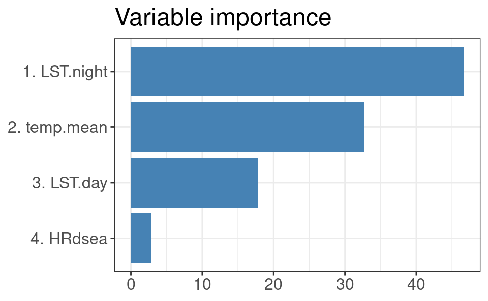

Figure 4.2: Variable importance for modeling spacetime daily temperatures.

We can use the fitted spacetime EML model to generate predictions e.g. for four consecutive days in August. First, we import MODIS LST for month of interest:

hrpred1km = hrgrid1km
sel.tifs1 = LST.listday[grep("_08_", LST.listday)]
sel.tifs2 = LST.listnight[grep("_08_", LST.listnight)]
## read to R in parallel
x1 = as.data.frame( parallel::mclapply(sel.tifs1, 
      function(i){x <- readGDAL(i)$band1; x <- ifelse(x<1, NA, x); return(x)}, 
                                       mc.cores = mc.cores))
x2 = as.data.frame( parallel::mclapply(sel.tifs2, 
      function(i){x <- readGDAL(i)$band1; x <- ifelse(x<1, NA, x); return(x)}, 
                                       mc.cores = mc.cores))
names(x1)  <- basename(sel.tifs1); names(x2) <- basename(sel.tifs2)

Second, we interpolate values between 8–day periods and fill gaps in EO data using simple linear interpolation (MODIS images are available only every 8 days):

dates.lst = as.Date("2006-08-13")+1:8
in.dates = c("2006-08-05", "2006-08-13", "2006-08-21", "2006-08-29")
in.days = as.numeric(strftime(as.Date(c(in.dates)), format = "%j"))
## interpolate values for missing dates in spacetime
library(parallel)
cl <- makeCluster(detectCores())
clusterExport(cl, c("in.days", "dates.lst"))
t1s = parallel::parApply(cl, x1, 1, 
      function(y) { try( approx(in.days, as.vector(y), xout=as.numeric(strftime(dates.lst, format = "%j")))$y ) })
t2s = parallel::parApply(cl, x2, 1, 
      function(y) { try( approx(in.days, as.vector(y), xout=as.numeric(strftime(dates.lst, format = "%j")))$y ) })
stopCluster(cl)
## remove missing pixels
x.t1s = parallel::mclapply(t1s, length, mc.cores = mc.cores)
t1s[which(!x.t1s==8)] <- list(rep(NA, 8))
t1s = do.call(rbind.data.frame, t1s)
names(t1s) = paste0("LST.day_", dates.lst)
x.t2s = parallel::mclapply(t2s, length, mc.cores = mc.cores)
t2s[which(!x.t2s==8)] <- list(rep(NA, 8))
t2s = do.call(rbind.data.frame, t2s)
names(t2s) = paste0("LST.night_", dates.lst)

Now we can make predictions for the target days in August 2006 by using (we run this operation in a loop to avoid RAM overload):

for(j in paste(dates.lst)){
  out.tif = paste0("output/MDTEMP_", j, ".tif")
  if(!file.exists(out.tif)){
    hrpred1km@data[,"LST.day"] = t1s[,paste0("LST.day_", j)]
    hrpred1km@data[,"LST.night"] = t2s[,paste0("LST.night_", j)]
    hrpred1km$temp.mean = temp.from.geom(fi=hrpred1km$Lat, 
                     as.numeric(strftime(as.Date(j), format = "%j")), 
                     a=37.03043, b=-15.43029, elev=hrpred1km$HRdem, t.grad=0.6)
    sel.pix = complete.cases(hrpred1km@data[,eml.TMP$features])
    out = predict(eml.TMP, newdata=hrpred1km@data[sel.pix,eml.TMP$features])
    hrpred1km@data[,paste0("MDTEMP_", j)] = NA
    hrpred1km@data[sel.pix, make.names(paste0("MDTEMP_", j))] = out$data$response * 10
    writeGDAL(hrpred1km[make.names(paste0("MDTEMP_", j))], out.tif, mvFlag = -32768,
              type = "Int16", options = c("COMPRESS=DEFLATE"))
  } else {
    hrpred1km@data[,make.names(paste0("MDTEMP_", j))] = readGDAL(out.tif)$band1
  }
}
#> output/MDTEMP_2006-08-14.tif has GDAL driver GTiff 
#> and has 487 rows and 490 columns
#> output/MDTEMP_2006-08-15.tif has GDAL driver GTiff 
#> and has 487 rows and 490 columns
#> output/MDTEMP_2006-08-16.tif has GDAL driver GTiff 
#> and has 487 rows and 490 columns
#> output/MDTEMP_2006-08-17.tif has GDAL driver GTiff 
#> and has 487 rows and 490 columns
#> output/MDTEMP_2006-08-18.tif has GDAL driver GTiff 
#> and has 487 rows and 490 columns
#> output/MDTEMP_2006-08-19.tif has GDAL driver GTiff 
#> and has 487 rows and 490 columns
#> output/MDTEMP_2006-08-20.tif has GDAL driver GTiff 
#> and has 487 rows and 490 columns
#> output/MDTEMP_2006-08-21.tif has GDAL driver GTiff 
#> and has 487 rows and 490 columns

To plot these predictions we can either put predictions in the spacetime package class (see gstat tutorial), or simply plot them using sp package:

st.pts = list("sp.points", idsta.pnts, pch = "+", col="black")
spplot(hrpred1km[make.names(paste0("MDTEMP_", dates.lst[c(1,4,8)]))], 
       col.regions=plotKML::R_pal[["rainbow_75"]][4:20],
       at = seq(143, 239, length.out=17),
       sp.layout = list(st.pts),
       main="Prediction daily temperature")
#dev.off()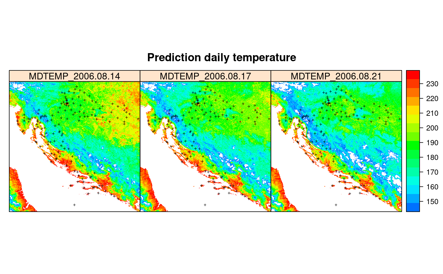

Figure 4.3: Predictions spacetime daily temperature for August 2006.

In summary, this example shows how to fit spatiotemporal EML with using also seasonality component together with the EO data. It can hence be considered a complete framework for spatiotemporal interpolation as both static, dynamic covariates and latitude / elevation are used for model training.

4.2 Spatiotemporal distribution of Fagus sylvatica

In the next example we show how to fit a spatiotemporal model using biological data: occurrences of Fagus sylvatica over Europe. This is the domain of Species Distribution modeling, except in this case we model distribution of target species also in spacetime. The training (point) data has been compiled for the purpose of the OpenDataScience.eu project, then cleaned and overlaid vs time-series of Landsat GLAD images and climatic variables (Bonannella et al., 2022; Witjes et al., 2022). For more details about the data refer also to the eumap repository.

We can load a snapshot of data by using:

library(data.table)
library(dplyr)
library(mlr)
library(sp)
fs.rm = readRDS('input/fagus_sylvatica_st.rds')
occ.pnts = fs.rm[,c("Atlas_class","easting","northing")]
coordinates(occ.pnts) = ~ easting + northing
proj4string(occ.pnts) = "+init=epsg:3035"
occ.pnts = spTransform(occ.pnts, CRS("+init=epsg:4326"))

This is a subset of a larger dataset that has been used to produce predictions of distribution of key forest tree species for Europe (you can browse the data via https://maps.opendatascience.eu). The first columns of this dataset show:

head(fs.rm[,1:10])
#>        id year postprocess Tile_ID easting northing Atlas_class lc1
#> 1  217127 2015   spacetime    4579 2925585  1639819           0    
#> 2 1078455 2007   spacetime   12496 3551500  2886500           1    
#> 3  332623 2012      yearly    8806 5650000  2286000           0 D20
#> 4  488689 2018      yearly   14583 4116000  3230000           0 B16
#> 5 2977316 2009   spacetime   23273 5376500  4601500           0    
#> 6  649000 2002   spacetime    8163 3286500  2211500           1    
#>   Abies_alba_distr.tiff Abies_spp._distr.tiff
#> 1                     0                     0
#> 2                   100                     0
#> 3                     0                     0
#> 4                   100                     0
#> 5                     0                     0
#> 6                     0                     0

The header columns are:

• id: is the unique ID of each point;
  
• year: is the year of obsevation;
  
• postprocess: column can have value yearly or spacetime to identify if the temporal reference of an observation comes from the original dataset or is the result of post-processing (yearly for originals, spacetime for post-processed points);
  
• Tile_ID: is as extracted from the 30-km tiling system;
  
• easting: is the easting coordinate of the observation point;
  
• northing: is the northing coordinate of the observation point;
  
• Atlas_class: contains name of the tree species or NULL if it’s an absence point coming from LUCAS;
  
• lc1: contains original LUCAS land cover classes or NULL if it’s a presence point;

Other columns are the EO and ecological covariates that we use for modeling distribution of Fagus sylvatica. We can plot distribution of points over EU using:

library(rnaturalearth)
library(raster)
europe <- rnaturalearth::ne_countries(scale=10, continent = 'europe')
europe <- raster::crop(europe, extent(-24.8,35.2,31,68.5))
#> Warning in .getSpatDF(x@ptr$df, ...): NAs introduced by coercion to integer
#> range

#> Warning in .getSpatDF(x@ptr$df, ...): NAs introduced by coercion to integer
#> range

#> Warning in .getSpatDF(x@ptr$df, ...): NAs introduced by coercion to integer
#> range

#> Warning in .getSpatDF(x@ptr$df, ...): NAs introduced by coercion to integer
#> range

#> Warning in .getSpatDF(x@ptr$df, ...): NAs introduced by coercion to integer
#> range

#> Warning in .getSpatDF(x@ptr$df, ...): NAs introduced by coercion to integer
#> range
op = par(mar=c(0,0,0,0))
plot(europe, col="lightgrey", border="darkgrey", axes=FALSE)
points(occ.pnts[occ.pnts$Atlas_class==1,], pch="+", cex=.8)
par(op)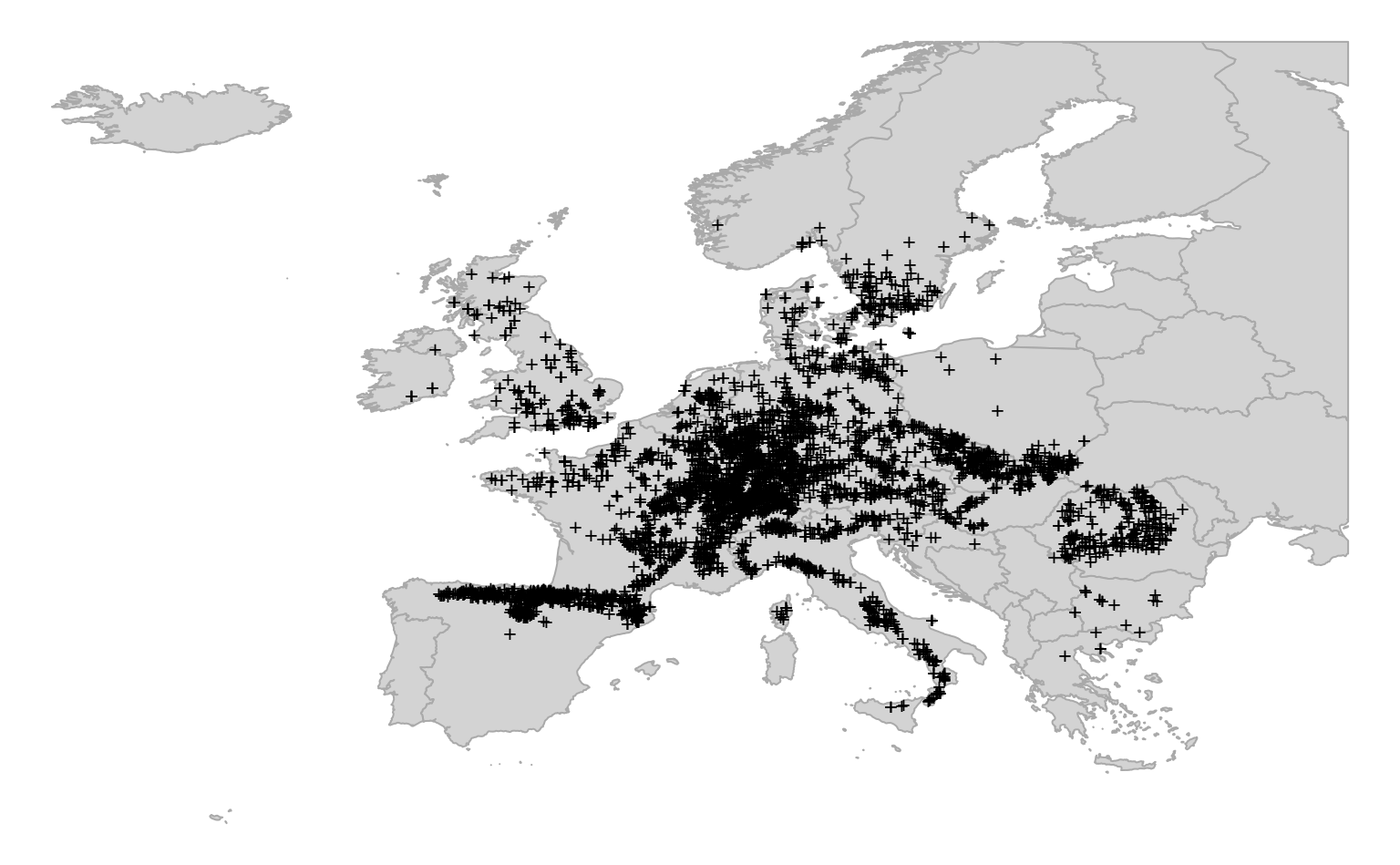

Figure 4.4: Distribution of occurrence locations for Fagus sylvatica. Each training points is also referrenced in time and hence can be used to run spacetime overlay.

As in previous examples, we first define the target model formula. We remove from model all other columns that are not used for prediction:

covs = grep("id|year|postprocess|Tile_ID|easting|northing|Atlas_class|lc1", 
          colnames(fs.rm), value = TRUE, invert = TRUE)
fm.fs = stats::as.formula(paste("Atlas_class ~ ", paste(covs, collapse="+")))
fs.rm$Atlas_class = factor(fs.rm$Atlas_class)
all.vars(fm.fs)[1:5]
#> [1] "Atlas_class"                    "Abies_alba_distr.tiff"         
#> [3] "Abies_spp._distr.tiff"          "Acer_campestre_distr.tiff"     
#> [5] "Acer_pseudoplatanus_distr.tiff"

To speed-up fitting of the models we have prepared two functions that wrap all modeling steps. First step consists of fine-tuning the base learners:

source("mlst_functions.R")
fs.rm0 = fs.rm %>% sample_n(5000)
tnd.ml = tune_learners(data = fs.rm0, formula = fm.fs, blocking = factor(fs.rm$Tile_ID))

This function runs hyperparameter optimization on binary classification models (classif.ranger, classif.xgboost, classif.glmnet) which will be later used to create an ensemble model. The intermediate models (fine-tuned RF and XGboost) are written to local folder output as RDS files. The output of the function is a RDS file including all the fine-tuned models and the formula.

The second step is the fitting of the ensemble model based on stacked regularization:

eml.fs = train_sp_eml(data = fs.rm0, tune_result = tnd.ml, blocking = as.factor(fs.rm$Tile_ID))

The function fits separately each of the previously used classification models: each algorithm will classify independently the probability of any training point being classified 0 (not-occurring) or 1 (occurring). The probability outputs of each model are then used as training dataset for the meta-learner. We use a GLM model with binomial link function (logistic regression):

#eml.fs = readRDS("output/eml_model.rds")
summary(eml.fs$learner.model$super.model$learner.model)
#> 
#> Call:
#> stats::glm(formula = f, family = "binomial", data = getTaskData(.task, 
#>     .subset), weights = .weights, model = FALSE)
#> 
#> Deviance Residuals: 
#>     Min       1Q   Median       3Q      Max  
#> -3.0986  -0.1150  -0.1123  -0.1122   3.1439  
#> 
#> Coefficients:
#>                 Estimate Std. Error z value Pr(>|z|)    
#> (Intercept)      -5.0655     0.1776 -28.527  < 2e-16 ***
#> classif.ranger    3.7088     0.6548   5.664 1.48e-08 ***
#> classif.xgboost   3.3720     0.5377   6.272 3.57e-10 ***
#> classif.glmnet    2.7881     0.2986   9.337  < 2e-16 ***
#> ---
#> Signif. codes:  0 '***' 0.001 '**' 0.01 '*' 0.05 '.' 0.1 ' ' 1
#> 
#> (Dispersion parameter for binomial family taken to be 1)
#> 
#>     Null deviance: 5314.27  on 4999  degrees of freedom
#> Residual deviance:  729.32  on 4996  degrees of freedom
#> AIC: 737.32
#> 
#> Number of Fisher Scoring iterations: 7

The variable importance analysis (RF component) shows that the most important covariates for mapping distribution of Fagus sylvatica are landsat images (which is expected considering the high spatial resolution) and the spatial distribution of other tree species (tree species commonly found together with Fagus sylvatica in the field):

library(ggplot2)
xl <- as.data.frame(mlr::getFeatureImportance(eml.fs[["learner.model"]][["base.models"]][[1]])$res)
xl$relative_importance = 100*xl$importance/sum(xl$importance)
xl = xl[order(xl$relative_importance, decreasing = T),]
xl$variable = paste0(c(1:238), ". ", xl$variable)
ggplot(data = xl[1:20,], aes(x = reorder(variable, relative_importance), y = relative_importance)) +
  geom_bar(fill = "steelblue",
           stat = "identity") +
  coord_flip() +
  labs(title = "Variable importance",
       x = NULL,
       y = NULL) +
  theme_bw() + theme(text = element_text(size=10))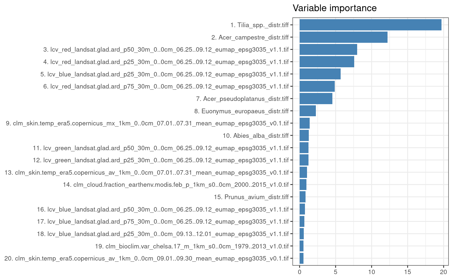

Figure 4.5: Variable importance for spatiotemporal model used to predict distribution of Fagus sylvatica.

To produce spacetime predictions for some tiles (30-m spatial resolution) we can run:

m1 = predict_tiles(input = "9690.2012",  model = eml.fs)
m2 = predict_tiles(input = "9690.2016",  model = eml.fs)
m3 = predict_tiles(input = "9690.2020",  model = eml.fs)
m1$Prob.2012 = m1$Prob
m1$Prob.2016 = m2$Prob
m1$Prob.2020 = m3$Prob

We can compare predictions of the probability of occurrence of the target species for two years next to each other by using:

pts = list("sp.points", spTransform(occ.pnts[occ.pnts$Atlas_class==1,], CRS("+init=epsg:3035")), 
           pch = "+", col="black")
spplot(m1[,c("Prob.2012","Prob.2016","Prob.2020")], names.attr = c("Prob.2010-2014", "Prob.2014-2018", "Prob.2018-2020"), col.regions=rev(bpy.colors()),
  sp.layout = list(pts),
  main="Realized distribution of Fagus sylvatica")

In this case there seems to be no drastic changes in the distribution of the target species through time, which is also expected because forest species distribution change on a scale of 50 to 100 year and not on a scale of few years. Some changes in distribution of the species, however, can be detected nevertheless. These can be due to abrupt events such as pest-pandemics, fires, floods or landslides or clear cutting of forests of course.

We can also plot the images using the plotKML package so that we can open and visualize predictions also in Google Earth or similar:

library(plotKML)
for(j in c(2012,2016,2020)){
  kml(m1, colour=m1@data[,paste0("Prob.", j)], file.name=paste0("prob.", j, ".kml"),
      raster_name = paste0("prob.", j, ".png"),
      colour_scale = SAGA_pal[["SG_COLORS_YELLOW_BLUE"]], 
      z.lim=c(0,100),
      TimeSpan.begin = as.Date(paste0(j, "-01-01")), TimeSpan.end = as.Date(paste0(j, "-12-31")))
}

In this case we attach to each prediction also the TimeSpan.begin and TimeSpan.end which means that Google Earth will recognize the temporal reference of the predictions. Opening predictions in Google Earth allows us to do some interpretation of produced maps and also analyze how much are the changes in vegetation cover connected with relief, proximity to urban areas, possible fire / flood events and similar.

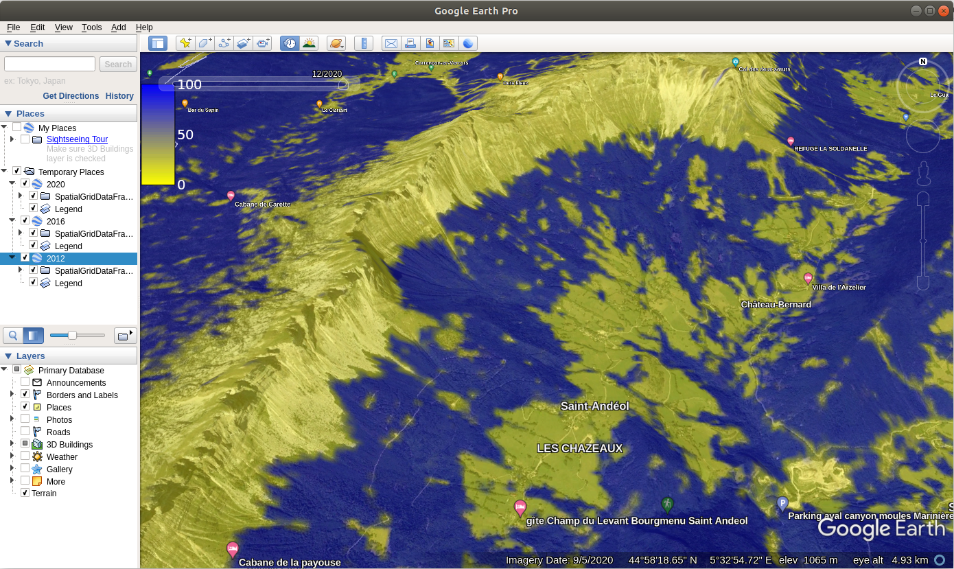
Figure 4.6: Spacetime predictions of distribution of Fagus Sylvatica visualized as time-series data in Google Earth.

We can check how the ensemble model performs in the classification task compared to the component models by running a resampling operation for each learner and the meta-learner. In this example we use a 5-fold spatial cross validation repeated 5 times. We first create new learners and assign the hyperparameters obtained from the fine-tuning operation:

learners = list(makeLearner("classif.ranger", predict.type = "prob", num.trees = 85),
                makeLearner("classif.xgboost", predict.type = "prob"),
                makeLearner("classif.glmnet", predict.type = "prob"))
learners[[1]] = mlr::setHyperPars(learners[[1]], par.vals = mlr::getHyperPars(tnd.ml[[1]]$learner))
learners[[2]] = mlr::setHyperPars(learners[[2]], par.vals = mlr::getHyperPars(tnd.ml[[2]]$learner))
learners[[3]] = mlr::setHyperPars(learners[[3]], par.vals = list(s = min(tnd.ml[[3]]$learner.model$lambda)))

Then we create the classification task (previously included in the functions), select which metric we want to evaluate our models on and resampling strategy. We are using logarithmic loss as performance metric for this example. After that, everything is set for the resampling operation, which we run in parallel:

#> Starting parallelization in mode=socket with cpus=32.
#> Exporting objects to slaves for mode socket: .mlr.slave.options
#> Resampling: repeated cross-validation
#> Measures:             logloss
#> Mapping in parallel: mode = socket; level = mlr.resample; cpus = 32; elements = 25.
#> 
#> Aggregated Result: logloss.test.mean=0.1131968
#> 
#> Exporting objects to slaves for mode socket: .mlr.slave.options
#> Resampling: repeated cross-validation
#> Measures:             logloss
#> Mapping in parallel: mode = socket; level = mlr.resample; cpus = 32; elements = 25.
#> 
#> Aggregated Result: logloss.test.mean=0.0818324
#> 
#> Exporting objects to slaves for mode socket: .mlr.slave.options
#> Resampling: repeated cross-validation
#> Measures:             logloss
#> Mapping in parallel: mode = socket; level = mlr.resample; cpus = 32; elements = 25.
#> 
#> Aggregated Result: logloss.test.mean=0.1695897
#> 

For the meta-learner, we access the predicted probabilities of the component models stored inside the ensemble model and use them as training data for the meta-learner in the resampling task. We need to create an additional task:

#> Exporting objects to slaves for mode socket: .mlr.slave.options
#> Resampling: repeated cross-validation
#> Measures:             logloss
#> Mapping in parallel: mode = socket; level = mlr.resample; cpus = 32; elements = 25.
#> 
#> Aggregated Result: logloss.test.mean=0.0743475
#> 
#> Stopped parallelization. All cleaned up.

Logloss is a robust metric when assessing performances of classification algorithms in the probability space. However, it is less intuitive to represent. To better compare performances across models, we standardize the logloss values according to the following equation:

\(R^2_\text{logloss} = 1 -\frac{Logloss_\text{m}}{Logloss_\text{r}}\)

Where \(Logloss_\text{m}\) is the logloss value of the model and \(Logloss_\text{r}\) is the logloss value of a model that performs no better than a random guess. We use the value of \(Logloss_\text{r}\) as a baseline for predictive performances. Values of \(R^2_\text{logloss}\) close to 1 indicate high predictive performances, while values close to 0 indicate poor predictive performances:

#>        RF       XGB       GLM       EML 
#> 0.7887610 0.8472908 0.6835250 0.8612585

From this example, we can see that the ensemble model outperforms, although slightly, all the other models. It is also interesting to notice how Random forest is the best component model if we look at the ensemble model coefficients, but in terms of performances Xgboost is actually the closest to the ensemble.

4.3 Summary notes

In this tutorial we have reviewed some aspects of spatial and spatiotemporal data and demonstrated how to use ML, specifically Ensemble ML, to train spatiotemporal models and produce time-series of predictions. We have also shown, using some synthetic and real-life datasets, how incorrectly setting up training and cross-validation can lead to over-fitting problems. This was done to help users realize that Machine Learning, however trivial it might seem, is not a click-a-button process and solid knowledge and understanding of advanced statistics (regression, hypothesis testing, sampling and resampling, probability theory) is still required.

For spatiotemporal models, we recommend combining covariates that can represent both long-term or accumulated effects of climate, together with covariates that can represent daily to monthly oscillation of variables such as soil moisture, temperatures and similar. During the design of the modeling system, we highly recommend trying to understand ecology and processes behind variable of interest first, then designing the modeling system to best reflect expert knowledge. The example with RF over-fitting data in Gasch et al. (2015) shows how in-depth understanding of the problem can help design modeling framework and prevent from over-fitting problems and similar. Witjes et al. (2022) and Bonannella et al. (2022) describe a more comprehensive framework for spatiotemporal ML which can even be run on large datasets.

Where time-series EO data exists, these can be also incorporated into the mapping algorithm as shown with three case studies. For spacetime overlays we recommend using Cloud-Optimized GeoTIFFs and the terra package (Hijmans, 2019) which helps speed-up overlays. Other options for efficient overlay are the stars and gdalcubes package (Appel & Pebesma, 2019).

Spatiotemporal datasets can be at the order of magnitude larger, hence it is important, when implementing analysis of spatiotemporal data, to consider computing optimization, which typically implies:

• Running operations in parallel;
• Separating fine-tuning and parameter optimization (best to run on subset and save computing time) from predictions,
• Using tiling systems to run overlay, predictions and visualizations,

Finally, we recommend following these generic steps to fit spatiotemporal models:

0. Define target of interest and design the modeling framework by understanding ecology and processes behind variable of interest.
   
1. Prepare training (points) data and a data cube with all covariates referenced in spacetime.
   
2. Overlay points in spacetime, create a spatiotemporal regression- or classification-matrix.
   
3. Add seasonal components, fine-tune initial model, reduce complexity as much as possible, and produce production-ready spatiotemporal prediction model (usually using Ensemble Machine Learning).
   
4. Run mapping accuracy assessment and determine prediction uncertainty including the per pixel uncertainty.
   
5. Generate predictions in spacetime — create time-series of predictions.
   
6. (optional) Run change-detection / trend analysis and try to detect main drivers of positive / negative trends (Witjes et al., 2022).
   
7. Deploy predictions as Cloud-Optimized GeoTIFF and produce the final report with mapping accuracy, variable importance.

Ensemble ML framework we used here clearly offers many benefits, but it also comes at a cost of at the order of magnitude higher computational load. Also interpretation of such models can be a cumbersome as there a multiple learners plus a meta-learner, so it often becomes difficult to track-back individual relationship between variables. To help increase confidence in the produced models, we recommend studying the Interpretable Machine Learning methods (Molnar, 2020), running additional model diagnostics, and intensively plotting data in space and spacetime and feature space.

Note that the mlr package is discontinued, so some of the examples above might become unstable with time. You are advised instead to use the new mlr3 package.